Tutorial Script – Lecture 6: Decisions
Date: Wednesday, 20 May 2026
Duration: 90 minutes
Lecture slides: AC_MS_6_Decisions.pdf (old lecture version — verify against new slides)
⚠️ Built from previous year’s lecture PDF — verify against new slides once available
0. Before the Tutorial (prep, not spoken)
What questions to expect:
- Students will conflate MT and LIP — this is the central confusion to resolve
- “What exactly is coherence?” — be ready with a crisp one-liner
- “Why saccades and not button presses?” — good metacognition question
- “What does 68 Hz actually mean?” — address: it’s an empirical average, not a fixed constant
- “Is the drift diffusion model just a metaphor?” — it’s mathematically precise, not just an analogy
Common misconceptions:
- LIP “makes” the decision — no, it represents the evolving decision variable; the threshold crossing triggers action
- MT and LIP are redundant — they encode fundamentally different quantities (instantaneous signal vs. accumulated evidence)
- Error trials mean LIP is “wrong” — LIP faithfully represents what the brain thinks, not the ground truth stimulus
- The 68 Hz threshold is a fixed biological constant — it is task-dependent and emerges from the RT paradigm only
Things to look up again before tutorial:
- Shadlen & Newsome (1996) PNAS — the original LIP delay task
- Shadlen & Newsome (2001) J Neurophysiol — LIP as temporal integrator, slopes
- Gold & Shadlen (2003) J Neurosci — FEF microstimulation experiment
- Britten et al. (1996) — ROC / choice probability analysis
1. Opening & Hook (5 min)
Set the scene without lecturing. Drop this quote on the board or say it aloud:
“The brain is a powerful decision-maker, able to form judgments about issues as simple as whether a sensory stimulus is present to those as complex as what career to choose or whom to marry. How are these judgments formed?”
— Gold & Shadlen (2001), TICS
Then immediately ask the group:
Opening question:
“Imagine you’re driving in heavy rain and you think you spot a friend by the roadside. You slow down, look longer, and eventually decide — yes or no. What is your brain actually doing during those extra seconds of looking? What changes between the first glance and the moment you decide?”
Let students answer freely for 2–3 min. Harvest keywords: uncertainty, more information, confidence, time. This primes the core lecture concept (evidence accumulation over time) without you having stated it yet.
2. Link to Last Week (5 min)
Last week: Mirror neurons — the brain represents observed actions of others in motor terms. The action observation system links perception to action.
This week: we go one step back. Before an action is selected, the brain must decide which action to take. We move from “observing actions” to “generating a decision that selects an action.”
Bridge sentence:
“Mirror neurons told us that perception and action are intimately linked in the brain. Today we ask: when the sensory input is ambiguous — when you’re not sure what you’re seeing — how does the brain resolve that ambiguity into a definite behavioral choice?“
3. The Paradigm: Random Dot Motion Task (10 min)
Core Message
The random dot motion (RDM) task is the key experimental tool for studying perceptual decisions. Understanding it in detail is the prerequisite for everything else.
Explanation Approach
Draw this on the board:
[Fixation point] → [Targets appear: T1 (left), T2 (right)] → [Random dots appear] → [Delay] → [Fixation off → Saccade]
Key parameters to convey:
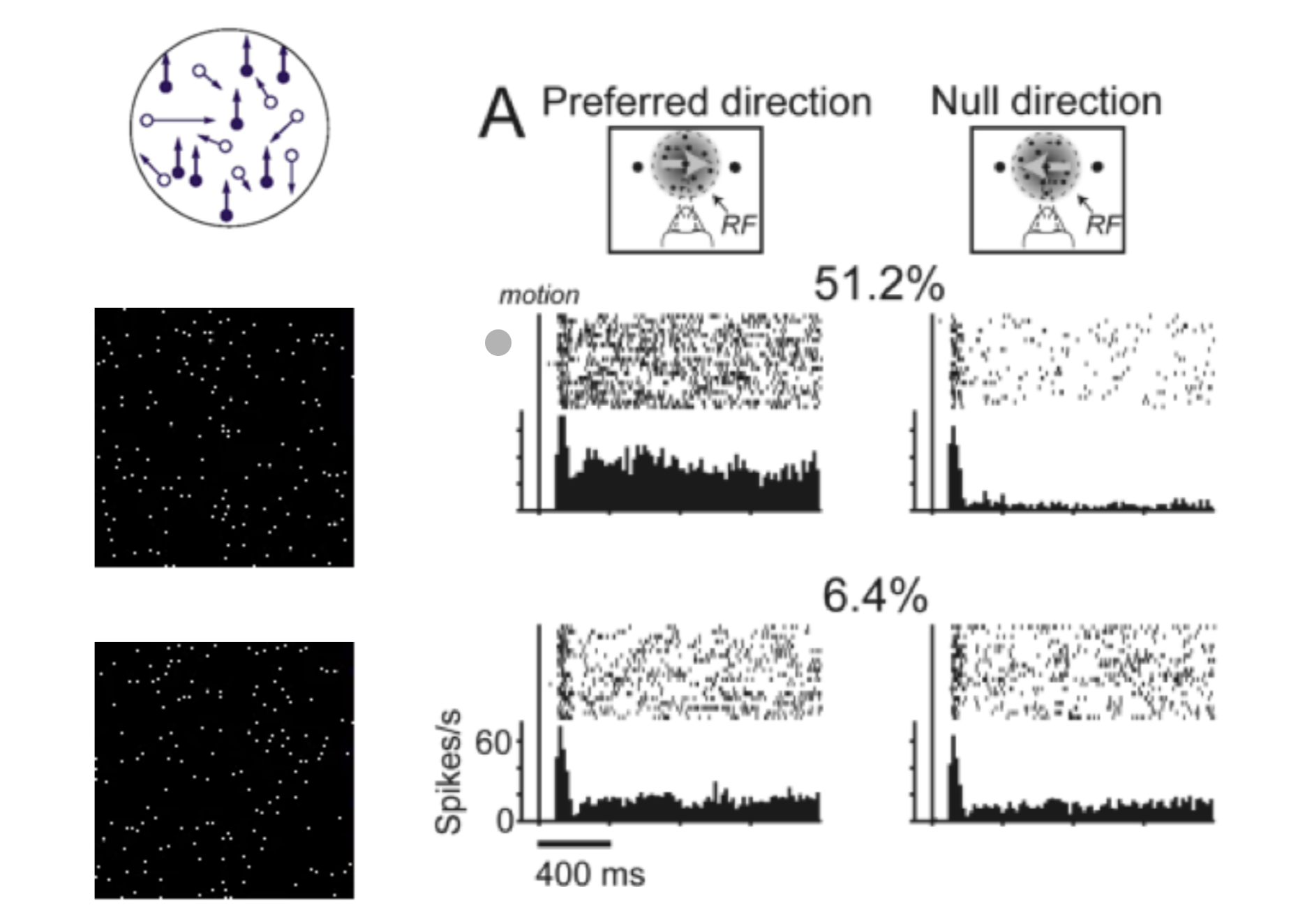
- A cloud of dots moves. Some percentage (coherence %) moves coherently in one direction; the rest moves randomly.
- 0% coherence = pure noise, chance performance
- 100% coherence = all dots move together, trivially easy
- The monkey reports its perceived direction with a saccade to the corresponding target
Why saccades? They are discrete, fast, spatially precise — ideal for neural recording. The oculomotor system is also well-mapped in non-human primates.
The key manipulation: coherence controls difficulty and therefore how much sensory evidence the brain must accumulate before deciding.
Discussion Questions
- Why is the coherence percentage such a powerful experimental variable — what exactly does varying it allow us to probe?
- Why is using saccades (eye movements) as the response measure such a methodological advantage compared to, say, a button press?
- If you ran this task on a human in an fMRI scanner, which brain areas would you predict to light up, and why?
Exam Relevance
- Exam Q1: “Describe the physiological basis of a decision process using the example of a random dot stimulus with a coherently moving subset of dots. Include a description of the role of different cortical areas in this process.” → This question requires describing the full paradigm + MT + LIP + threshold.
4. Area MT: Encoding Instantaneous Sensory Evidence (10 min)
Core Message
MT (Middle Temporal area) encodes the current motion signal — fast, transient, stimulus-locked. It does NOT accumulate information over time.
Explanation Approach
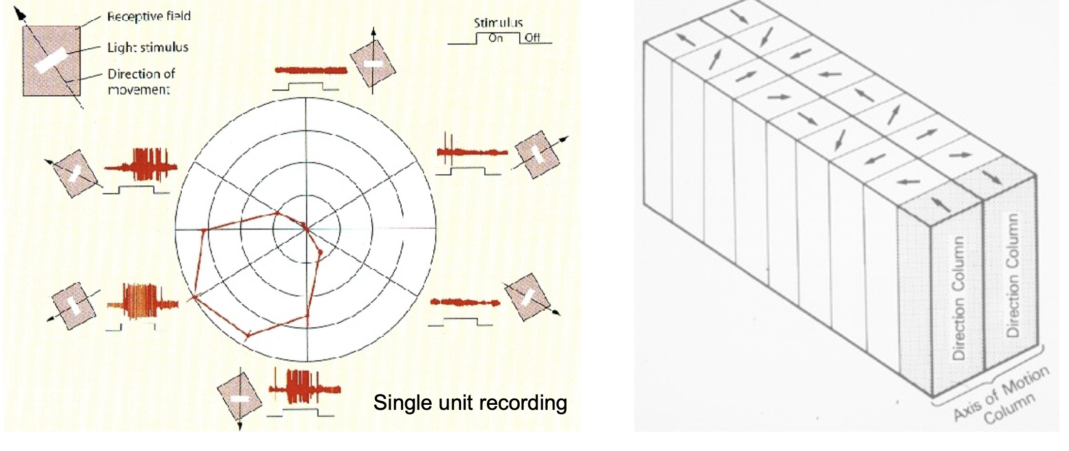
Key MT properties (flashback):
- Large receptive fields sensitive to direction and speed of motion
- Neurons arranged in direction hypercolumns (analogous to orientation columns in V1)
- Response scales with coherence level — more coherent motion in preferred direction → higher firing rate
- Critical property: once the stimulus disappears, MT goes silent. It represents momentary evidence only.
The lecture notes: “MT represents the direction and coherence of the random dot stimulus.”
Analogy: MT is like a weather vane — it tells you the current wind direction accurately, but the moment the wind shifts, it shifts too. It has no memory.
Discussion Questions
- MT neurons are organized in direction columns. How does this architecture make MT well-suited to represent motion direction, and what would be the consequence of damaging MT?
- The activation of MT scales with coherence — but at 0% coherence, there is still some MT activity. What does that tell us?
- If MT only encodes instantaneous evidence, what kind of downstream structure would you need to make a decision based on MT output over time?
Common Misconceptions
- “MT makes the decision” → MT is only the sensory input stage. It has no persistent activity and no threshold mechanism.
- “MT is silent at 0% coherence” → Even random noise activates MT neurons (noise has local motion signals); the population is just not systematically biased.
Exam Relevance
- Exam Q3: “Describe qualitative differences in the activity patterns of neurons in MT and LIP in a motion discrimination task.” → MT = fast/transient/stimulus-locked; LIP = slow/ramping/decision-locked.
5. ROC Analysis: How Well Does MT Predict the Decision? (8 min)
Core Message
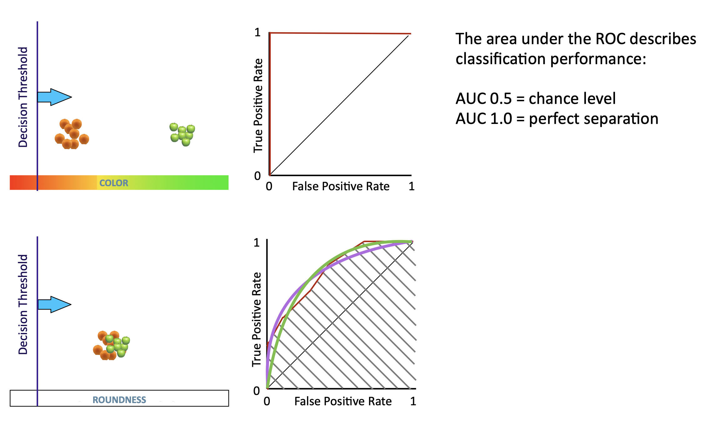
ROC (Receiver Operator Characteristic) analysis quantifies how well a neuron’s firing rate predicts behavioral outcome — it is a parameter-free, elegant tool.
Explanation Approach
The lecture introduces ROC via the fruit-sorting analogy: imagine sorting apples by roundness. If roundness perfectly separates apples from non-apples, AUC = 1.0; if it’s useless, AUC = 0.5.
Apply this to neuroscience:
- Take an MT neuron. On trials where the monkey chose T1, what was its firing rate? On trials where it chose T2?
- The distributions overlap — but by how much?
- Choice probability (Britten et al. 1996): AUC of the ROC when comparing “chosen preferred” vs. “chosen null” trials
- d’ = 1.0 → perfect prediction
- d’ = 0.5 → random
- d’ = 0.0 → always wrong (worse than chance — also informative!)
Key result: MT activity correlates with the monkey’s choice, not just the stimulus. Even at a fixed coherence, when the monkey chose T1 vs T2, MT firing rates differ slightly. This suggests MT contributes probabilistically to the decision.
Discussion Questions
- Why is it important that ROC/AUC is parameter-free — what would be the risk of using a threshold-dependent measure instead?
- A choice probability of exactly 0.5 for an MT neuron would mean what about its relationship to the decision?
- Why does the false positive rate matter in a different way for “Is this car coming toward me?” vs. “Is this defendant guilty?” — and how does this relate to what the threshold does in the decision model?
Common Misconceptions
- “ROC analysis is only for medical tests” → It is a general tool for any binary classification problem, used extensively in neurophysiology.
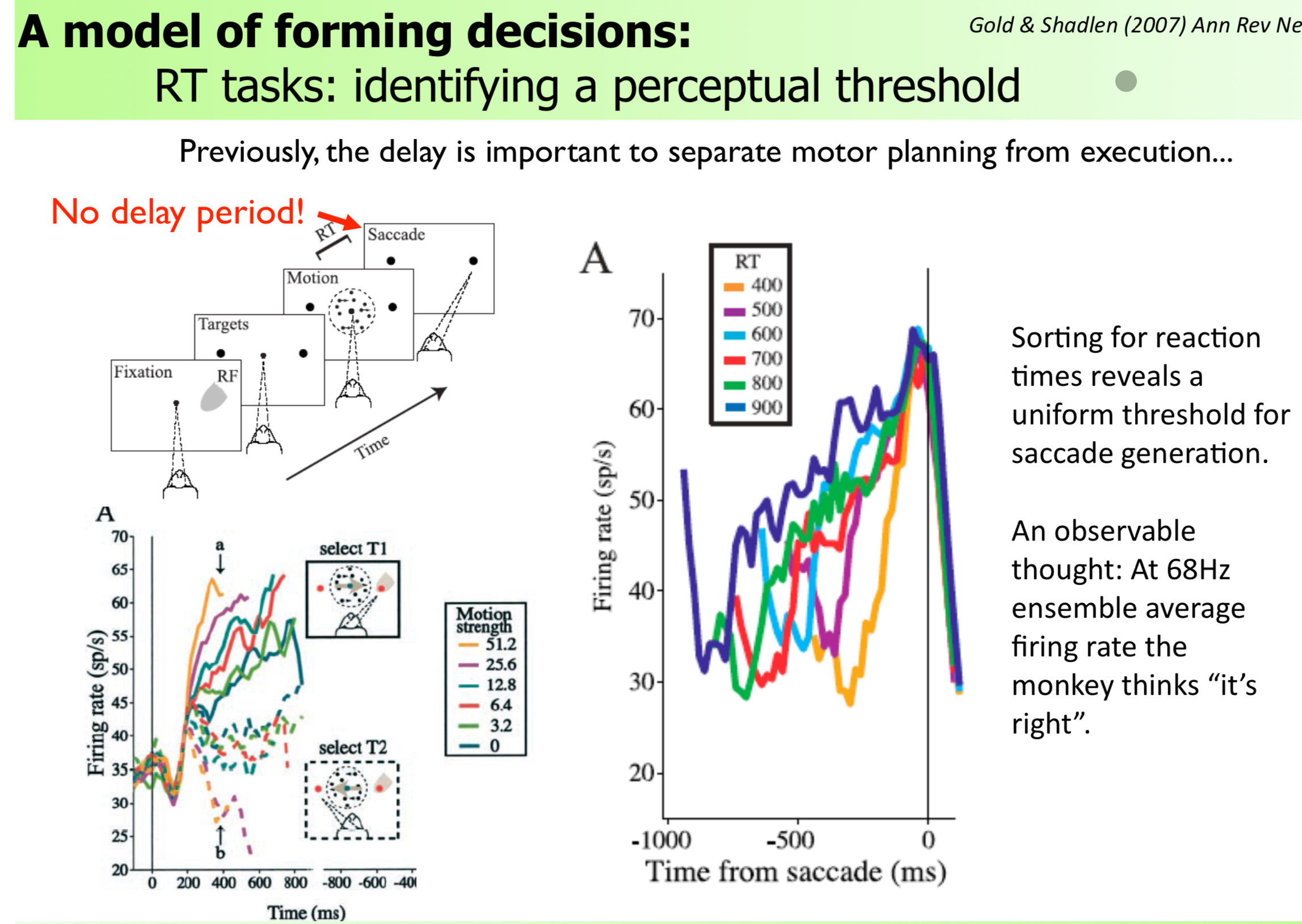
6. Area LIP: Integrating Evidence Over Time (15 min)
Core Message
LIP (Lateral Intraparietal Cortex) is the neural substrate of the decision variable — it accumulates evidence from MT over time, ramping up until a threshold is crossed.
Explanation Approach
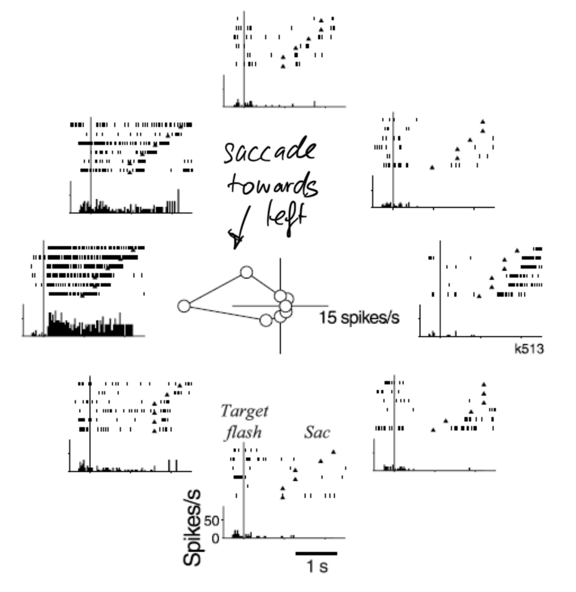
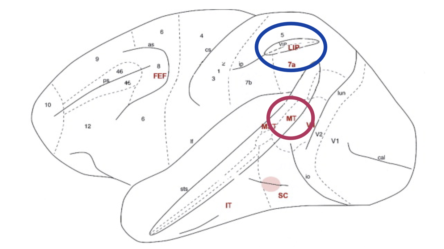
Start with the anatomical point: LIP sits in parietal cortex, downstream of MT in the dorsal stream. LIP neurons have saccade target fields — each neuron represents a potential saccade target location.
The delay task (Shadlen & Newsome 1996, 2001):
- Monkey views RDM stimulus for fixed duration, then a delay period, then saccade
- During motion viewing: LIP neurons ramp up gradually — higher coherence = steeper slope
- During delay period: activity is maintained even after the dots are gone → this is motor planning, not sensory encoding
- At saccade initiation: activity drops back to baseline
Critical contrast with MT:
| Property | MT | LIP |
|---|---|---|
| What it encodes | Instantaneous motion signal | Accumulated evidence (decision variable) |
| Response profile | Fast, transient, stimulus-locked | Slow, ramping, persistent in delay |
| At 0% coherence | Symmetric noise | Still ramps — based on noise! |
| After stimulus off | Silent | Maintained (motor plan) |
The lecture’s key line: “Evidence is momentary, the decision variable evolves over time.”
Analogy: If MT is a weather vane, LIP is a rain gauge — it accumulates drop by drop. The weather vane resets with every gust, but the rain gauge remembers.
Key formula-free summary of what LIP computes:
LIP ≈ ∫(MT_preferred − MT_null) dt
It approximates the integral of the difference between competing MT pools (one favoring left, one favoring right).
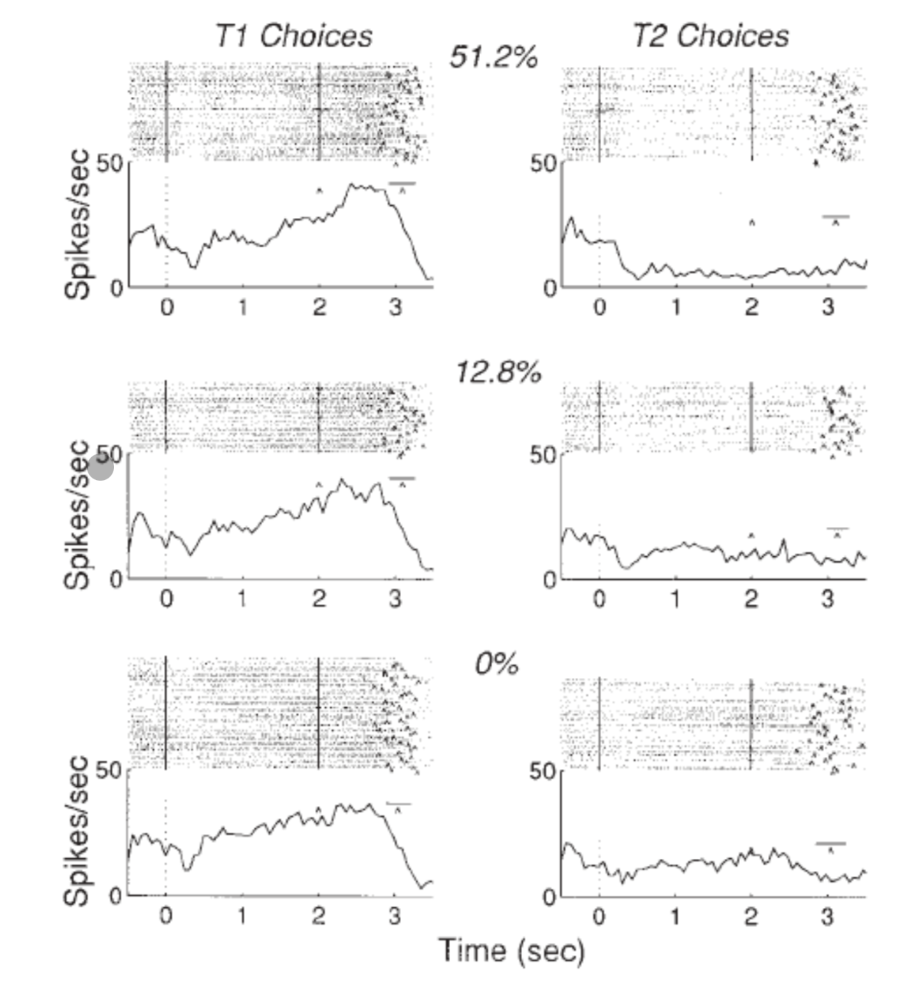
Error trials
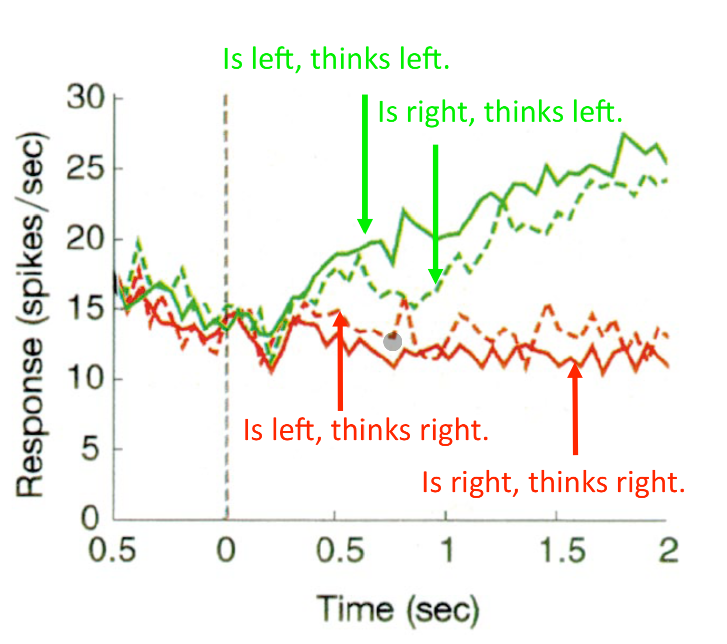
This is a conceptually important result:
- On error trials, the stimulus moves rightward but the monkey reports leftward
- LIP neuron activity ramps toward T1 (left) — the wrong target
- Conclusion: LIP activity represents what the monkey believes, not what the stimulus actually is
- The decision process is running correctly; it is the evidence input that was noisy/unlucky
“Reading the monkey’s mind: if you look at LIP, you know not what the dots are doing, but what the monkey thinks the dots are doing.”
Discussion Questions
- LIP activity ramps even at 0% coherence — decisions can be made based purely on noise. What does this imply about the brain’s decision process in situations where there is genuinely no signal?
- How does the delay period help us experimentally dissociate the motor planning phase from the actual movement execution?
- Given that LIP represents the decision variable and not the stimulus, what does this say about where in the processing hierarchy the “real” decision is being made?
Common Misconceptions
- “LIP activity causes the monkey to be right or wrong” → Causality: LIP represents the evolving decision; it doesn’t cause the accuracy, which depends on what MT happened to feed into it
- “The delay period is just waiting” → It is the window where motor preparation happens in the absence of ongoing sensory evidence — theoretically crucial
Exam Relevance
- Exam Q2: “Describe the pattern of activity of a representative LIP neuron in a motion discrimination task. Also consider error trials.”
- Exam Q3: MT vs. LIP qualitative differences
- Exam Q4: “Describe the classical paradigm, i.e. the experimental design, which is used to measure the importance of LIP neurons in decision processes.”
Interactive: LIP Predictive Index Simulation
The plot below mirrors Shadlen & Newsome (2001) Fig. 7. It shows how well LIP activity at each moment in time can predict which target the monkey will ultimately choose. AUC = 0.5 means chance (no predictive information); AUC → 1.0 means perfect prediction.
How to read it: higher coherence means steeper rise = the decision is readable earlier from LIP activity. All curves converge to a high AUC by the end of the motion epoch.
# Pyodide / Obsidian Execute Code: install matplotlib first.
import micropip
await micropip.install("matplotlib")

import numpy as np
import matplotlib.pyplot as plt

rng = np.random.default_rng(42)
dt = 0.025
t_max = 2.0
n_steps = int(t_max / dt)
t_full  = np.arange(n_steps) * dt
noise, n_trials = 0.6, 150  # 150 preferred + 150 null per coherence level

def erf_poly(x):
    a = np.abs(x)
    t = 1.0 / (1.0 + 0.3275911 * a)
    poly = t * (0.254829592 + t * (-0.284496736 + t * (1.421413741
               + t * (-1.453152027 + t * 1.061405429))))
    val = 1.0 - poly * np.exp(-a**2)
    return np.where(x >= 0, val, -val)

def normal_auc(pos_vals, neg_vals):
    if len(pos_vals) < 2 or len(neg_vals) < 2:
        return 0.5
    sp = np.std(pos_vals, ddof=1); sn = np.std(neg_vals, ddof=1)
    pooled = np.sqrt((sp**2 + sn**2) / 2)
    if pooled < 1e-6: return 0.5
    d_prime = (np.mean(pos_vals) - np.mean(neg_vals)) / pooled
    return float(0.5 * (1.0 + erf_poly(d_prime / (2.0 * np.sqrt(2.0)))))

def simulate_batch(drift):
    """Simulate preferred-direction (+drift) and null-direction (-drift) trials.
    AUC between these two groups mirrors the LIP predictive index from S&N 2001."""
    pref = np.zeros((n_trials, n_steps))
    null = np.zeros((n_trials, n_steps))
    for j in range(n_trials):
        for i in range(1, n_steps):
            e1 = noise * np.sqrt(dt) * rng.normal()
            e2 = noise * np.sqrt(dt) * rng.normal()
            pref[j, i] = np.clip(pref[j, i-1] + drift * dt + e1, -1.5, 1.5)
            null[j, i] = np.clip(null[j, i-1] - drift * dt + e2, -1.5, 1.5)
    return pref, null

coherences = [0.0, 0.25, 0.5, 0.9, 1.6]
coh_labels = ['0%', '~6%', '~13%', '~26%', '~51%']
colors     = ['#999999', '#4477aa', '#66aadd', '#ee8833', '#cc2222']

fig, ax = plt.subplots(figsize=(10, 5))
for drift, col, lab in zip(coherences, colors, coh_labels):
    pref, null = simulate_batch(drift)
    pred = [normal_auc(pref[:, i], null[:, i]) for i in range(n_steps)]
    ax.plot(t_full, pred, color=col, lw=2.0, label=f'coherence ≈ {lab}')

ax.axhline(0.5, color='gray', ls=':', lw=1.2, alpha=0.7, label='chance (0.5)')
ax.axvline(1.5, color='black', ls='--', lw=1.0, alpha=0.5, label='approx. delay onset')
ax.set_xlabel("Time into motion epoch (s)", fontsize=12)
ax.set_ylabel("Predictive index (AUC)", fontsize=12)
ax.set_title("LIP Predictive Index Over Time\n"
             "Mirrors Shadlen & Newsome (2001) Fig. 7 — slope ∝ coherence", fontsize=12)
ax.legend(title='Coherence', fontsize=9, loc='upper left')
ax.set_ylim(0.4, 1.05); ax.grid(alpha=0.3)
plt.tight_layout(); plt.show()
🤖 AI addition (15/06/26): Fixed bug in original code. Original used a single positive drift for all trials, so at high coherence nearly all trials ended positive → the “null choice” group was empty → AUC broke down. Fix: simulate preferred (+drift) and null (−drift) direction trials separately per coherence level. AUC is now computed between these two stimulus classes at each timepoint, which correctly captures how discriminable preferred vs. null LIP trajectories are over time.
Q: What does it mean that all curves reach approximately the same AUC level by the delay period? Does coherence affect when the decision is final, or how confident it is?
Coherence primarily affects when the decision becomes readable, not the asymptotic level of certainty. By the end of the motion epoch, LIP activity has had enough time to accumulate even weak evidence to a similar ceiling — the decision is equally “locked in” for all coherence levels (AUC ≈ 0.9–1.0). What differs is how fast each curve gets there: high coherence crosses the decision threshold early in the epoch; low coherence needs the full duration.
This matches the DDM prediction exactly: drift rate changes RT, not accuracy at long viewing times. A slow integrator given enough time is as accurate as a fast one. The practical implication is that coherence determines whether a decision is ripe at 300 ms or needs 2 s — the brain is doing the same computation either way, just at different speeds. This is also why the delay period activity looks similar across coherences: by the time the dots turn off, the evidence race is essentially over for all conditions.
7. The Drift Diffusion Model (8 min)
Core Message
The drift diffusion model (DDM) provides a mathematically precise, unified account of both accuracy and reaction time in perceptual decisions.
Explanation Approach
The model in plain English:
- Imagine a particle on a line between two walls (+B and -B)
- The particle drifts in the direction supported by the evidence (coherence determines drift rate)
- Random noise makes the path meandering — like Brownian motion
- When the particle hits a wall → decision made for that alternative
- B controls the speed-accuracy tradeoff: larger B → more accurate, slower; smaller B → faster, more errors
The RT task version (Shadlen & Newsome 2001):
In the reaction time (RT) task, there is no fixed delay — the monkey saccades when ready.
- Higher coherence → steeper slope in LIP → threshold reached faster → shorter RT
- Same threshold (~68 Hz average firing rate) regardless of coherence
- The slope varies; the endpoint (threshold) is constant
Key quote from lecture: “Sorting for reaction times reveals a uniform threshold for saccade generation. At 68 Hz ensemble average firing rate the monkey thinks ‘it’s right’.”
⚠️ Fact-check: The 68 Hz figure is a population average from Shadlen & Newsome (2001), not a universal biological constant. The lecture is correct to note it is task-dependent. Do not teach it as a fixed threshold across all monkeys or tasks.
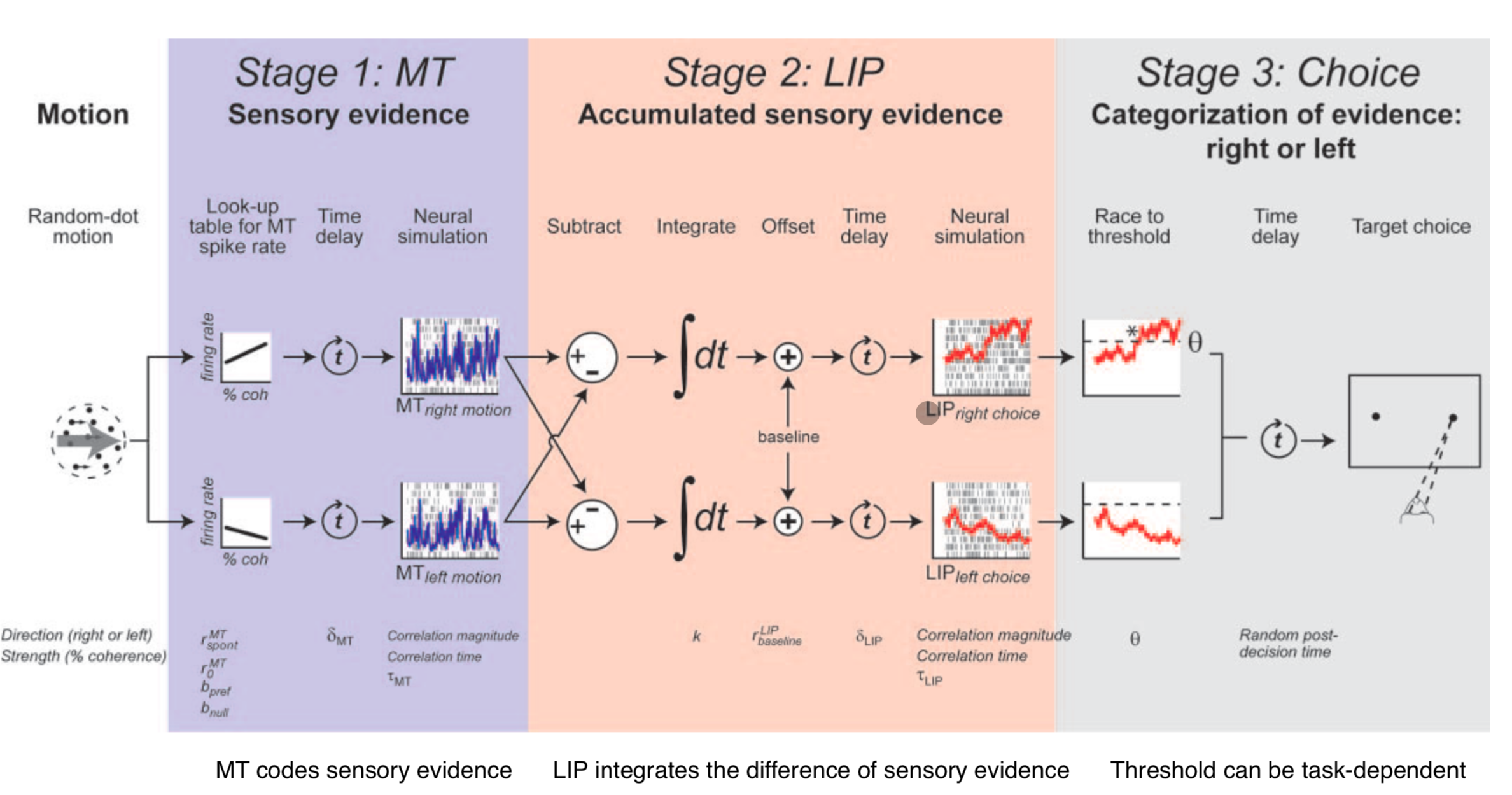
The complete model hierarchy:
- MT codes sensory evidence (input layer)
- LIP integrates the difference of sensory evidence (integrator)
- Threshold → action selection (output)
This is a general model — not limited to dot motion and saccades. The architecture (detect signal → integrate evidence → threshold for action) applies broadly.
Discussion Questions
- The drift diffusion model predicts both accuracy and RT from a single set of parameters. Why is this elegant — what would it mean if you needed two separate models?
- In the RT task, steeper LIP slopes lead to faster decisions. But does steeper always mean “more correct”? When would faster be wrong?
- How does the threshold parameter B relate to real-world decision strategies — think of a doctor deciding whether to prescribe a drug, vs. a sprinter responding to the starting gun?
Exam Relevance
- Exam Q (implicit from Q1 and Q4): Explaining why RT decreases with coherence in terms of the model
- The complete model slide is explicitly marked “Most important slide” in the lecture PDF
8. FEF Microstimulation: Reading the Evolving Decision (12 min)
Core Message
FEF (Frontal Eye Fields) microstimulation experiments demonstrated that the oculomotor system has access to the ongoing decision process — not just its final outcome. This is causal evidence.
Explanation Approach
Context: FEF is in frontal cortex, contains a topographic map of saccade targets. Stimulating FEF electrically triggers saccades — it is part of the oculomotor output system.
The experiment (Gold & Shadlen 2003, J Neurosci):
Setup:
- Monkey fixates, targets appear, RDM stimulus shown
- During the motion viewing period, LIP is recorded
- After the dots disappear (during delay), FEF is microstimulated
- This evokes an involuntary saccade — but its direction is not random
What they found:
- The involuntary saccade is systematically biased toward the target the monkey was planning to choose
- The size of the bias depends on:
- Coherence level (more coherence → stronger bias)
- Viewing time (longer viewing → stronger bias)
- At low coherence or short viewing time: little bias (nascent decision is weak)
- At high coherence or long viewing time: strong bias (decision is well-formed)
Control condition: When FEF was stimulated without a concurrent decision being formed (no RDM stimulus), the involuntary saccade was not systematically biased — it went in the FEF’s preferred direction only.
The key conceptual result:
“The oculomotor system is informed about the evolving decision, not just the final post-threshold outcome of the decision process.”
This is inconsistent with a serial model where: [sensory processing] → [decision completed] → [motor command issued]. Instead, decision formation and motor preparation overlap continuously in time.
Why this is marked “Most important slide”: It provides causal evidence (via stimulation) that the motor system tracks the decision variable as it builds up — blurring the line between “deciding” and “acting.”
Discussion Questions
- The FEF experiment is correlational in one sense (LIP activity correlates with the upcoming saccade) but manipulative in another (FEF stimulation biases the saccade). What is the epistemological advantage of the manipulative component?
- This result is “inconsistent with the notion that a central decision maker completes its operation before activating the motor structures.” What alternative architecture does it suggest?
- What would it mean for free will and conscious decision-making if the motor system is already acting on an evolving decision before that decision is consciously experienced?
Common Misconceptions
- “FEF makes the decision” → FEF is part of the oculomotor output; it reads the decision from LIP, it does not compute it
- “Microstimulation results are clean” → The stimulated saccade is involuntary and superimposed on the monkey’s planned saccade; the separation requires careful analysis
Exam Relevance
- Exam Q6: “FEF was micro-stimulated. Explain the experimental setup and tell the results.”
- Marked “Most important slide” in the lecture
9. Perceptual Decisions in Humans (5 min)
Core Message
The monkey RDM findings generalize to humans — analogous areas (DLPFC, FFA/PPA) show the same evidence accumulation pattern.
Explanation Approach
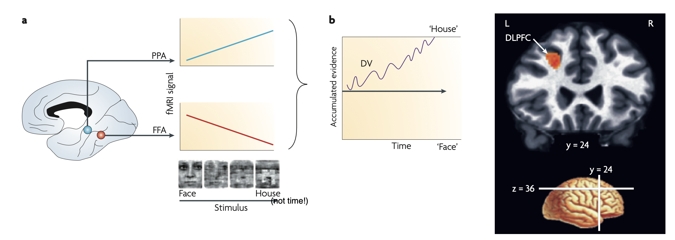
Heekeren et al. (2008) Nat Rev Neurosci used a face-house categorization task in fMRI:
- FFA (fusiform face area) represents face evidence; PPA (parahippocampal place area) represents house evidence
- DLPFC computes the difference between FFA and PPA activity → the decision variable
- DLPFC activity ramps toward the correct category during accumulation, analogous to LIP in monkeys
Human analogue of RDM: degraded images of faces/houses with varying noise levels — the “coherence” is replaced by image clarity.
The key lecture question: “What is a nice analogue in humans for the random dot motion stimuli used so much in monkeys?” → Degraded/noisy visual images of meaningful categories.
ℹ️ Note: The specific homology of DLPFC (humans) ↔ LIP (monkeys) is suggested by functional similarity, not established by direct anatomical tracing. The lecture presents this as the current best understanding.
Discussion Questions
- How does using the face-house task allow researchers to study evidence representation in humans in a way that is impossible with the pure RDM task?
- DLPFC in humans is implicated in many executive functions beyond decision-making. How do you think researchers control for this when interpreting fMRI results from a decision task?
10. Exam Question Round (15 min)
Work through these with the group — have students answer first, then refine together.
Question 1: (Exam Q1) Describe the physiological basis of a decision process using the example of a random dot stimulus with a coherently moving subset of dots. Include a description of the role of different cortical areas in this process.
Key points of a good answer:
- Describe the RDM paradigm: variable coherence, saccade response
- MT: encodes current motion direction; firing rate scales with coherence; transient/stimulus-locked
- LIP: integrates difference of MT signals over time; firing rate ramps monotonically; slope steeper with higher coherence; maintained activity in delay
- Threshold: when LIP reaches ~68 Hz (in RT task), saccade is initiated
- The complete model: MT (detect) → LIP (integrate) → threshold → action
- Error trials: LIP ramps for the wrong target, but faithfully represents the monkey’s internal belief
Typical mistakes:
- Describing MT and LIP as doing the same thing
- Saying LIP “detects” motion — it integrates, not detects
- Forgetting the delay period and what it reveals
Question 2: (Exam Q3) Describe qualitative differences in the activity patterns of neurons in MT and LIP in a motion discrimination task.
Key points:
- MT: fast response, transient, stops when stimulus stops, proportional to current coherence
- LIP: slow ramp, persists through delay, slope is a function of coherence, threshold-triggered
- LIP at 0% coherence: still ramps (based on noise → still makes a decision)
- MT is a “sensor”, LIP is an “integrator/decision variable”
Typical mistakes:
- Saying LIP responds faster
- Not mentioning the delay period maintenance of LIP
Question 3: (Exam Q6) FEF was microstimulated. Explain the experimental setup and results.
Key points:
- Monkey views RDM, forms nascent decision; FEF is stimulated after stimulus offset
- Stimulation evokes involuntary saccade
- Involuntary saccade is biased toward monkey’s planned target (systematic separation)
- Bias scales with coherence and viewing time
- Conclusion: FEF (oculomotor system) has access to the ongoing decision process, not just the final outcome
- This is evidence against a strictly sequential model of decide-then-act
Typical mistakes:
- Confusing FEF stimulation with LIP recording
- Saying FEF “makes” the decision
- Missing the key conclusion about continuous (not post-threshold) motor access to the decision variable
Closing (3 min)
Take-Home Message:
“A decision is not an event — it is a process. MT tells the brain what is happening right now; LIP accumulates that signal over time into a growing certainty; and the motor system is watching LIP the whole time, ready to act the moment the evidence tips over threshold. The brain doesn’t wait to finish deciding before it starts preparing to move.”
Preview of next week (Lecture 7: Plasticity):
How does the brain change as a result of experience? After studying how decisions guide actions, we ask: what happens to the neural circuits that mediate those actions when they are practiced repeatedly? The motor cortex we studied in Lecture 4 turns out to be remarkably plastic — and the mechanisms of that plasticity are directly relevant to motor learning, rehabilitation, and skill acquisition.
Quick Reference: Key Papers
| Paper | Key result |
|---|---|
| Shadlen & Newsome (1996) PNAS | Basic decision task; LIP activity ramps during motion viewing |
| Shadlen & Newsome (2001) J Neurophysiol | LIP as temporal integrator; RT task with slopes |
| Gold & Shadlen (2003) J Neurosci | FEF microstimulation; continuous motor access to decision |
| Britten et al. (1996) Visual Neurosci | Choice probability via ROC analysis |
| Heekeren et al. (2008) Nat Rev Neurosci | Human decision-making; face-house task; DLPFC |
| Gold & Shadlen (2007) Ann Rev Neurosci | RT task threshold identification |
Timing Overview
| Block | Topic | Time |
|---|---|---|
| 1 | Opening & hook | 5 min |
| 2 | Link to last week | 5 min |
| 3 | RDM paradigm | 10 min |
| 4 | MT area | 10 min |
| 5 | ROC analysis | 8 min |
| 6 | LIP + error trials | 15 min |
| 7 | Drift diffusion model | 8 min |
| 8 | FEF microstimulation | 12 min |
| 9 | Humans | 5 min |
| 10 | Exam Q round | 15 min |
| — | Closing | 3 min |
| Total | ~96 min |
Trim ROC or Humans section if running long — they are lower exam priority.