Attention Mechanism

methods-of-ai ai-generated

The attention mechanism lets every token in a sequence look at every other token and pull in the information it needs. Each token produces a Query, a Key, and a Value (via learned matrices); the attention weight from one token to another is a deterministic function of how well its query matches the other’s key. It is the core of the Transformer (Transformers) — and, in the exam paper, the operation that implements exponential path-merging.

No randomness

Attention does not pick partners by chance. Given the input and the (trained) weights, the whole computation is deterministic — same input → same attention pattern every time. (The random rollouts you may be thinking of belong to Monte Carlo Tree Search, not attention.)

The idea: Query · Key · Value

Each token’s embedding is projected three ways through learned weight matrices W_Q, W_K, W_V:

	Meaning	Question it answers
Query Q	what this token is looking for	”what do I need?”
Key K	what this token offers	”what do I have?”
Value V	the content it passes on if attended to	”what I hand over”

Q = X · W_Q      K = X · W_K      V = X · W_V

where X = the matrix of token embeddings (one row per token).

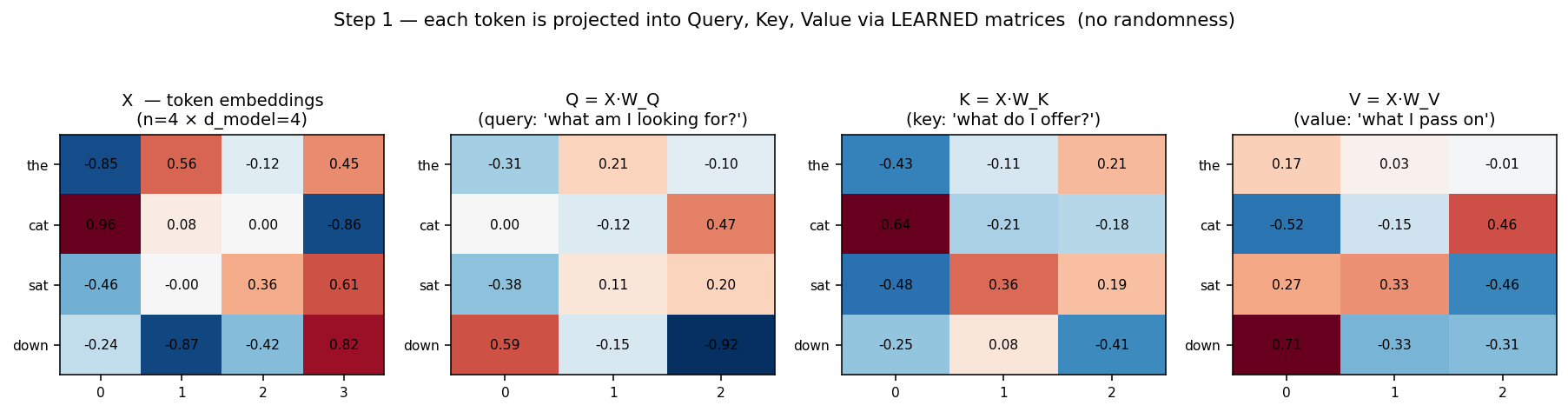
Each of the 4 tokens (“the”, “cat”, “sat”, “down”) becomes a row; multiplying by the learned matrices gives the Q, K, V matrices. The weights are fixed after training — this projection is pure linear algebra, no chance involved.

The formula

$\text{Attention}(Q,K,V)=\underset{\text{attention weights }A}{\underbrace{\text{softmax}\left(\frac{Q{K}^{\top }}{\sqrt{d_k}}\right)}}V$

Step by step:

1. Scores = Q·Kᵀ — dot product of every query with every key → an n × n matrix of “match strengths.”
2. Scale by 1/√d_k — keeps the numbers from blowing up as dimension grows (stops softmax from saturating).
3. Softmax over each row → the attention weights A. Each row sums to 1 (a probability distribution over “where this token looks”).
4. Multiply by V → each token’s output is a weighted blend of all values, weighted by attention.

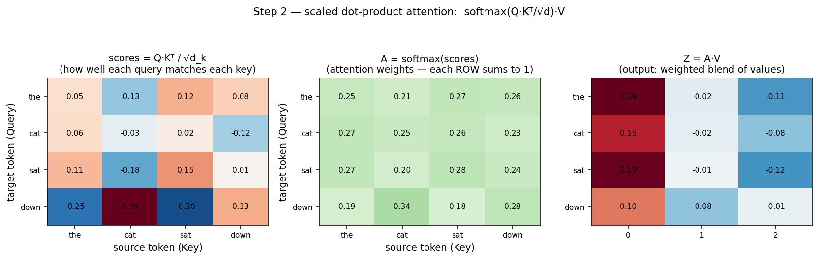
Left: raw match scores Q·Kᵀ/√d (red = strong match, blue = weak). Middle: after softmax, each row is a distribution summing to 1 — e.g. “down” attends most to “cat” (0.34). Right: the output Z = A·V, each token now a blend of the values it attended to.

Reading the attention matrix

The n × n matrix A is the heart of it: row i = how token i spreads its attention over all tokens (including itself).

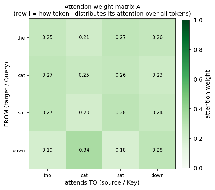
Row = the target (the token doing the querying, “FROM”); column = the source (the token being attended to, “TO”). Bright = strong attention. In the paper’s terms, an attention operation is one bright cell: source token i → target token j.

(Here the embeddings were random, so attention is near-uniform — in a trained model these rows become sharply peaked on the relevant tokens. See the next example for what “trained” looks like.)

Example 2 — sharp, interpretable attention

The example above was random → near-uniform. A trained model learns Q/K so that each token attends almost entirely to the one token it needs. Here Q, K, V are hand-designed to encode a little syntactic story:

Token	attends to	(why)
the → cat	94.8 %	determiner → its noun
cat → sat	94.8 %	subject → its verb
sat → cat	94.8 %	verb → its subject
down → sat	94.8 %	adverb → its verb

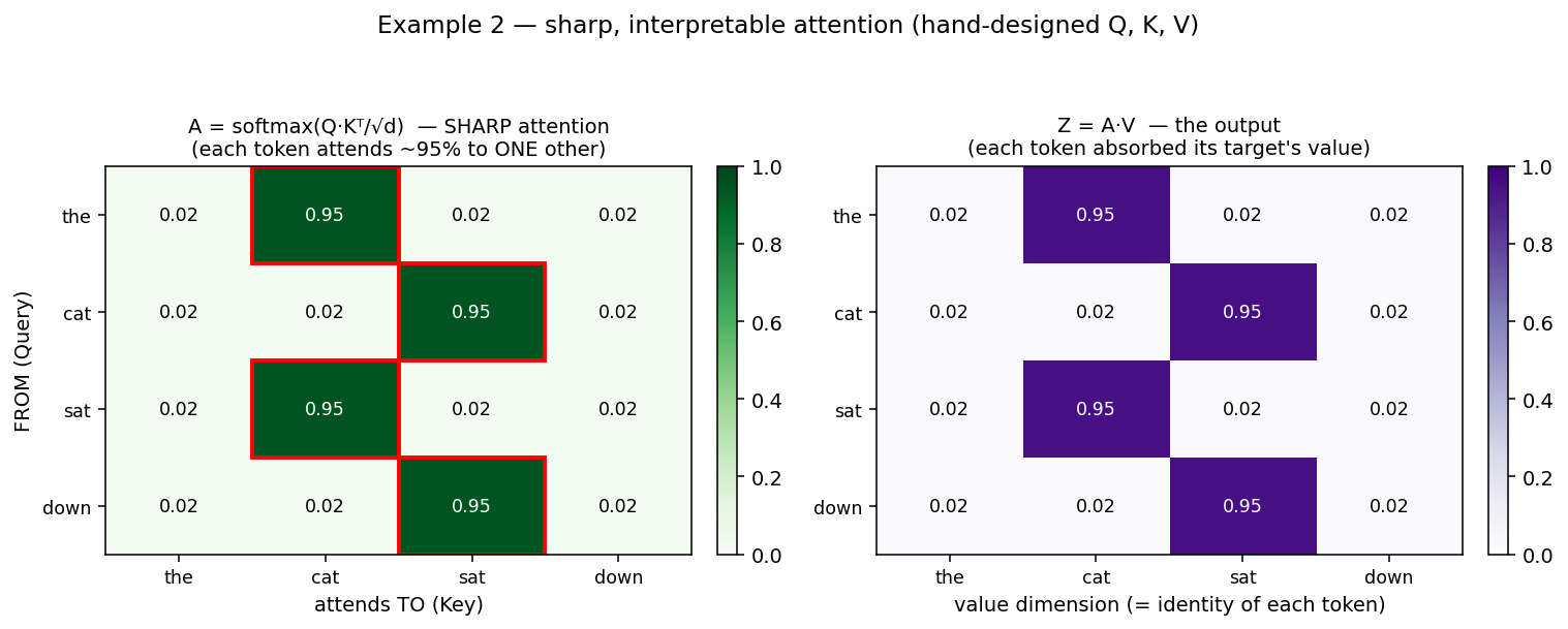
Left (A): each row is now sharply peaked — ~95 % of the attention goes to one token (red boxes = the learned dependency), only ~1.7 % leaks to each other token. Right (Z = A·V): since each token’s value was set to its own identity, the output shows each token has absorbed the value of the token it attended to — e.g. “the” ‘s output row is ~95 % the cat dimension. That’s the whole point of attention: information flows from the attended token into the attending one.

How it’s engineered (so you can see there’s no magic): make each token’s Key a distinct strong direction (K = 8·I), and each token’s Query point exactly at its target’s key direction. Then Q·Kᵀ is large only at the target → softmax concentrates there. A real model learns W_Q/W_K to do this.

targets = {0:1, 1:2, 2:1, 3:2}        # the->cat, cat->sat, sat->cat, down->sat
K = 8 * np.eye(4)                      # distinct, strong keys  -> sharp softmax
Q = np.zeros((4,4))
for i,t in targets.items(): Q[i,t] = 1 # each query points at its target's key
V = np.eye(4)                          # value = identity, so output shows what was absorbed
A = softmax(Q @ K.T / np.sqrt(4))      # -> 94.8% on the target, 1.7% elsewhere

The contrast in one glance

Random weights → flat attention (~0.25 everywhere, useless). Trained/structured weights → peaked attention (~0.95 on the right token). Learning attention is learning to make the right Q·K dot products large. In the paper, “learning to search” = learning W_Q/W_K so a vertex’s query matches the key of the right frontier vertex.

The runnable core (Python)

import numpy as np
def softmax(z):
    e = np.exp(z - z.max(axis=1, keepdims=True))
    return e / e.sum(axis=1, keepdims=True)
 
X   = np.random.uniform(-1, 1, (4, 4))     # 4 tokens, d_model = 4
W_Q = np.random.uniform(-1, 1, (4, 3))     # project to d_k = 3
W_K = np.random.uniform(-1, 1, (4, 3))
W_V = np.random.uniform(-1, 1, (4, 3))
 
Q, K, V = X @ W_Q, X @ W_K, X @ W_V
scores  = Q @ K.T / np.sqrt(3)             # n x n match scores
A       = softmax(scores)                  # attention weights, rows sum to 1
Z       = A @ V                            # output: n x d_k
assert np.allclose(A.sum(axis=1), 1)       # every row is a distribution

Matrix shapes (the bit that’s easy to lose)

For n tokens, model dim d_model, projected dim d_k:

Object	Shape
X (embeddings)	n × d_model
W_Q, W_K, W_V	d_model × d_k
Q, K, V	n × d_k
scores = Q·Kᵀ	n × n
A = softmax(scores)	n × n
output Z = A·V	n × d_k

⚠️ The n × n score matrix is why attention is O(n²) in sequence length — the well-known cost that motivates long-context tricks.

Multi-head attention (one line)

Instead of one attention, run h of them in parallel with separate W_Q/W_K/W_V (“heads”), then concatenate. Each head can specialise on a different relation (syntax, position, coreference…). The paper’s models use 1 head per layer deliberately, to make the circuit easy to reverse-engineer.

Connection to the exam paper — attention as path-merging

In Saparov et al., each vertex token stores the set of vertices reachable from it, and one attention operation per layer performs a path-merge:

• Q of vertex j: “give me the reachable set of a vertex I can reach.”
• K of vertex i: “I am vertex v.”
• High Q·K → j attends to i → copies i’s reachable set (the V) into its own.

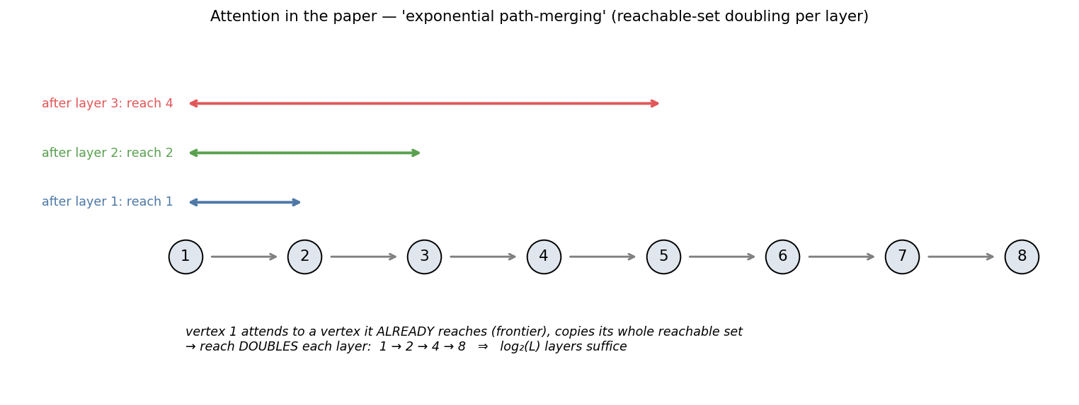
Layer 1: a vertex matches along direct edges (finds its children). Deeper layers: it matches along reachability — it attends to a vertex it already reaches (possibly far away) and absorbs that vertex’s whole reachable set. So the reach doubles per layer (1→2→4→8) instead of growing by 1 → only log₂(L) layers are needed. (This edge-vs-reachability distinction is exactly why it’s log-depth, not linear.)

One-liner for the oral

“Attention: each token makes a Query, Key, Value via learned matrices; the weight from token j to token i is softmax(Qⱼ·Kᵢ/√d) — deterministic, not random. In the paper, a vertex’s query matches the key of a frontier vertex it already reaches, copying that vertex’s reachable set (the value) — and because it merges with far vertices, the reach doubles per layer, giving log-depth path-merging.”

See also

• Transformers · exponential path-merging · Selection-Inference · Monte Carlo Tree Search
• pruefung_paper-transformers-search_25-05-26 (exam dossier — §4 path-merging, §3 mechanistic method)
• Neural Networks & Deep Learning
• Superlink: Methods of AI Lecture

Created: 01/06/26