Markov Decision Process (MDP)

Markov Decision Process (MDP) — Planning II

chatbot methods-of-ai

Companion files for exam prep:

• 📋 lernzettel_planning-ii_30-04-26 — compact 1-page exam sheet
• ✏️ quiz_planning_30-04-26 — 8 questions (shared with Planning I)
• 🔗 lernzettel_planning-i_30-04-26 — sibling: Planning I (Classical / STRIPS)

Table of contents

1. Core Ideas
2. Mini-glossary
3. MDP Formal Definition
4. Markov Property
5. Policies
6. Expected & Discounted Rewards
7. Bellman Equation
8. Bellman Optimality Equation
9. Grid World — worked example
10. Playing with the Rewards
11. Formulas & Notation
12. Common Exam Traps
13. Quick Comparison Tables
14. ALGORITHMS ⭐ — pseudocode for all 6
    • Policy Evaluation · Policy Improvement · [[#3-policy-iteration-|Policy Iteration ⭐]]
    • Value Iteration · Modified Policy Iteration · Linear Programming
15. Algorithm comparison table
16. Original atomic-note context · MDP ↔ RL · Python gridworld code · Where MDPs are used today · Where MDPs were extended — and by what

---

Core Ideas

• Classical planning assumes deterministic actions. MDPs handle uncertainty (stochastic outcomes) AND long-term consequences.
• An MDP assigns a probability to each outcome of each action, and a reward for each state-action pair.
• The goal is to find an optimal policy π — a mapping from states to actions that maximizes expected (discounted) reward.
• Key property: Markov = future depends only on the current state and action, not the full history.
• “Reasoning about policies” splits into three subproblems of increasing difficulty (slide 38):
  1. Given MDP + policy → evaluate policy.
  2. Given MDP → find optimal policy.
  3. Find optimal policy for unknown MDP → reinforcement learning (next session).

---

Mini-glossary

Term	Meaning
State s ∈ S	A configuration the agent can be in (e.g. grid position).
Action a ∈ A	A move the agent can attempt.
Transition p(s’|s, a)	Probability of landing in s’ after performing a in s.
Reward r(s, a)	Short-term benefit of performing a in s.
Policy π : S → A	Deterministic mapping: which action to take in each state.
Value function V^π(s)	Expected discounted reward starting in s and following π.
Optimal value V*(s)	Value achieved by an optimal policy from s.
Discount factor γ	Real number between 0 and 1 weighting future rewards.
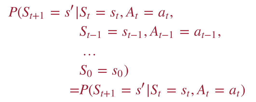
Markov property	P(Sₜ₊₁ | Sₜ, Aₜ, history) = P(Sₜ₊₁ | Sₜ, Aₜ).
Episode	A trajectory s₀, a₀, r₀, s₁, a₁, r₁, …

---

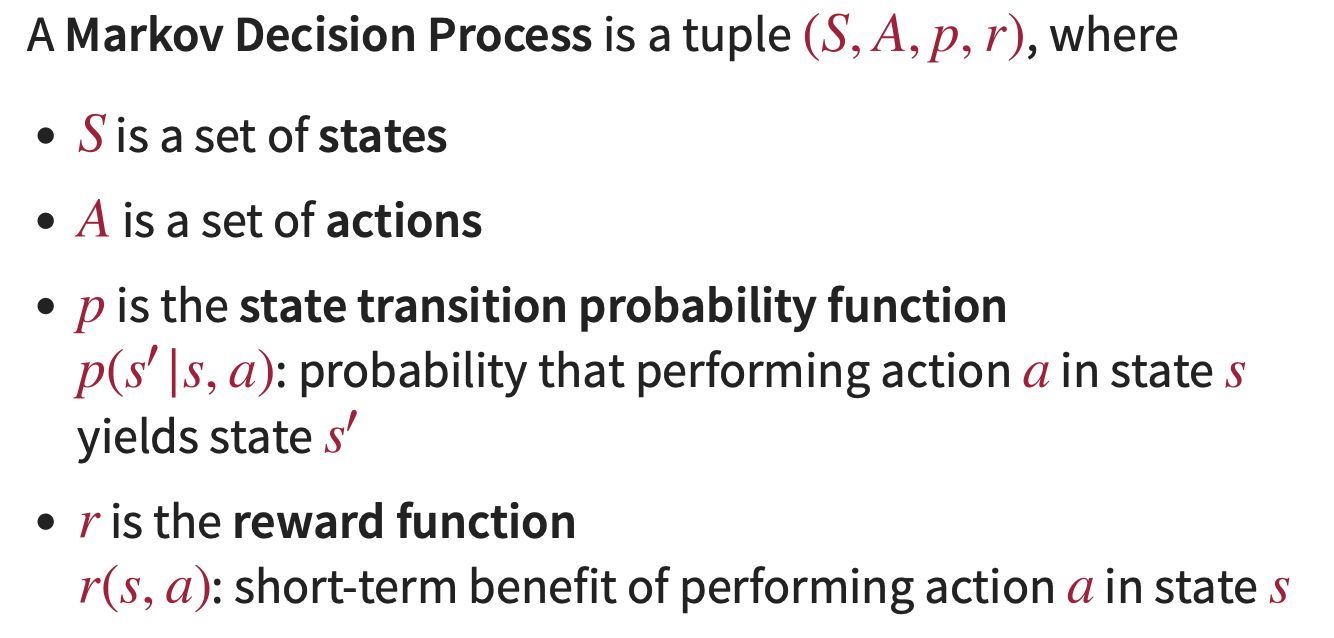
MDP Formal Definition

A Markov Decision Process is a tuple (S, A, p, r) (slide 14):

• S — set of states
• A — set of actions
• p(s’|s, a) — state transition probability function
• r(s, a) — reward function (short-term benefit of action a in state s)

⚠️ γ is NOT part of the tuple. The discount factor is a parameter of the evaluation criterion, not of the MDP itself. The same MDP can be solved with different γ values yielding different optimal policies.

(Quiz Q117 / Q119 hammer this point.)

---

Markov Property

“Markov” generally means: given the present, the future and the past are independent.

For MDPs specifically:

$$\begin{array}{rl}& P(S_{t+1}=s^{\prime }\mid S_t=s_t,A_t=a_t,S_{t-1}=s_{t-1},A_{t-1}=a_{t-1},\dots ,S_0=s_0)\\ & =P(S_{t+1}=s^{\prime }\mid S_t=s_t,A_t=a_t)\end{array}$$

Just like in classical search: the successor function depends only on the current state.

Why this matters: if the property holds, we can build a tractable solver — policies depend only on the current state, not the full history of how we got here.

---

Policies

• A (deterministic Markov) policy assigns an action to each state: π : S → A.
• It is defined for every state — not just the start state. (This is the key difference to a classical plan, which is a single sequence of actions for one initial state.)
• A policy can be visualised in Grid World as an arrow in every cell.

Example:

• π((1,1)) = up
• π((1,2)) = up
• π((3,1)) = left ← surprising! see Grid World

---

Expected & Discounted Rewards

When following policy π, we can compute the probability P(Sₖ = s) of being in state s at the k-th step. The expected reward at step k is:

${\mathbb{E}}_{\pi }[r_k]={\sum }_{s}P(S_k=s)\cdot r(s,\pi (s))$

The (undiscounted) expected reward of policy π is the (possibly infinite) series:

${\mathbb{E}}_{\pi }[r_1]+{\mathbb{E}}_{\pi }[r_2]+{\mathbb{E}}_{\pi }[r_3]+\dots$

Why discount?

• Future rewards may be less valuable (economics).
• To guarantee convergence of the infinite series.

γ-discounted reward

${\mathbb{E}}_{\pi }[r_1]+\gamma \cdot {\mathbb{E}}_{\pi }[r_2]+{\gamma }^2\cdot {\mathbb{E}}_{\pi }[r_3]+{\gamma }^3\cdot {\mathbb{E}}_{\pi }[r_4]+\dots$

where γ is a real number between 0 and 1 (slide 34 — inclusive endpoints).

• γ close to 0 → short-sighted agent.
• γ close to 1 → long-term planner.
• γ = 1 is explicitly allowed but the value series may be unbounded if there is no terminal state (slide 67 — “termination problem”).

Example (slide 35). For γ = 0.5 the first four terms are r₁, 0.5·r₂, 0.25·r₃, 0.125·r₄ (the weight halves with every future step).

---

Bellman Equation (Policy Evaluation)

For a fixed policy π, the value of state s satisfies:

$V^{\pi }(s)=r(s,\pi (s))+\gamma {\sum }_{s^{\prime }}p(s^{\prime }\mid s,\pi (s))V^{\pi }(s^{\prime })$

This is a linear system of |S| equations in |S| unknowns. Two ways to solve it:

1. Solve the linear system directly (e.g. matrix inversion).
2. Iterate — see [[#1. Policy Evaluation (iterative Bellman)|Algorithm #1]].

---

Bellman Optimality Equation

The optimal value function V* satisfies:

$V^{\ast }(s)={\max }_a\left[r(s,a)+\gamma {\sum }_{s^{\prime }}p(s^{\prime }\mid s,a)V^{\ast }(s^{\prime })\right]$

The key difference from the Bellman equation: instead of plugging in π(s) we maximise over all actions. This system is non-linear (because of the max) — that is why Value Iteration is the natural fit (it does the max inside the update).

Once V* is known, an optimal policy is recovered greedily:

${\pi }^{\ast }(s)={\mathrm{argmax}}_a\left[r(s,a)+\gamma {\sum }_{s^{\prime }}p(s^{\prime }\mid s,a)V^{\ast }(s^{\prime })\right]$

---

Grid World — worked example

Setup (slide 17 ff.).

• 4 × 3 grid, one wall cell at (2, 2). Start = (1, 1).
• States S = {(1,1), (2,1), (3,1), (4,1), (1,2), (3,2), (4,2), (1,3), (2,3), (3,3), (4,3)}.
• Actions A = {up, down, left, right}.
• Two terminal states with absorbing rewards: (4, 3) → +1, (4, 2) → −1.
• All other states have step reward r(s, a) = −0.04.

Stochastic transitions (slide 20).

• With probability 0.8 the intended direction is taken.
• With probability 0.1 the agent moves 90° clockwise to the intended direction.
• With probability 0.1 the agent moves 90° counter-clockwise.
• If a move would leave the grid or hit the wall: agent stays put.

Concrete transitions for s = (1, 1) (slide 23):

Query	Value
p((1,2) | (1,1), up)	0.8
p((1,1) | (1,1), left)	0.8 (left) + 0.1 (down) = 0.9
p((1,3) | (1,1), up)	0
p((2,1) | (1,1), up)	0.1

Optimal policy & values (γ = 1, slide 40 ff.):

	col 1	col 2	col 3	col 4
row 3	→ 0.812	→ 0.868	→ 0.918	+1
row 2	↑ 0.762	wall	↑ 0.660	−1
row 1	↑ 0.705	← 0.655	← 0.611	← 0.388

Subtle observations (worth the exam):

• (1, 2) has higher value than (2, 1): going right risks slipping into the −1 trap. Going up is safer.
• Optimal policy at (3, 1) is left (back toward start), not up. Reason: if “up” misfires and the agent slips right, it lands in (4, 1) which has the worst non-terminal value (0.388, close to the −1 trap). Going left is the safer detour.
• Optimal policy at (2, 1) is left (back to start). Going to start gives expected value 0.705, which is 0.094 higher than continuing toward (3, 1) at 0.611 — worth the detour.

Playing with the rewards (slides)

The step reward profoundly changes the optimal policy:

Step reward r	Behaviour
−2 (heavy penalty)	Each step costs more than reaching any goal. Optimal: end the game ASAP, even via the −1 trap (e.g. from (3, 2) the policy is “right” into the −1).
−0.4 (moderate)	Intermediate: still go up from (1, 1), but from (2, 1) go right to avoid long detours.
−0.04 (default)	The 0.812/0.762/… policy above — risk-averse, avoids the trap with a detour.

(Positive step rewards are not discussed in the slides — they would incentivise the agent to wander forever, which only makes sense with γ < 1 to keep the value bounded. Background, not a slide claim.)

---

Visualisations (Python)

The four figures below illustrate the classic 4×3 R&N Grid World end-to-end: the reward layout, a hand-computed optimal policy, the value function produced by Value Iteration, and the convergence rate of VI itself. All implemented in pure Python — numpy is used only for plotting convenience, the MDP solver is plain dicts and lists.

🐍 Figure 1 — Grid World layout with rewards

import micropip
await micropip.install("matplotlib")
 
import matplotlib.pyplot as plt
from matplotlib.patches import Rectangle
 
# 4 cols × 3 rows. Coordinates: (col, row) with row 1 at the bottom (R&N convention).
COLS, ROWS = 4, 3
WALL = (2, 2)
GOAL = (4, 3)       # +1
TRAP = (4, 2)       # -1
STEP_REWARD = -0.04
 
def reward(cell):
    if cell == GOAL: return 1.0
    if cell == TRAP: return -1.0
    if cell == WALL: return None
    return STEP_REWARD
 
fig, ax = plt.subplots(figsize=(8, 6))
 
# Build a colour for each cell from its reward
for c in range(1, COLS + 1):
    for r in range(1, ROWS + 1):
        cell = (c, r)
        x, y = c - 1, r - 1
        if cell == WALL:
            ax.add_patch(Rectangle((x, y), 1, 1, facecolor="black",
                                   edgecolor="white", lw=2))
            ax.text(x + 0.5, y + 0.5, "WALL", ha="center", va="center",
                    color="white", fontweight="bold", fontsize=11)
            continue
        rew = reward(cell)
        if cell == GOAL:
            fc = "#27ae60"
        elif cell == TRAP:
            fc = "#e74c3c"
        else:
            fc = "#ecf0f1"
        ax.add_patch(Rectangle((x, y), 1, 1, facecolor=fc,
                               edgecolor="black", lw=2))
        label = f"{cell}\nr = {rew:+.2f}"
        text_col = "white" if cell in (GOAL, TRAP) else "black"
        ax.text(x + 0.5, y + 0.5, label, ha="center", va="center",
                color=text_col, fontsize=10, fontweight="bold")
 
ax.set_xlim(0, COLS); ax.set_ylim(0, ROWS)
ax.set_aspect("equal"); ax.set_xticks([]); ax.set_yticks([])
ax.set_title("Grid World (R&N 4×3) — reward layout\n"
             "green = +1 goal · red = −1 trap · grey = −0.04 step cost · black = wall",
             fontsize=11)
plt.tight_layout(); plt.show()

What this figure shows. The classic 4×3 Russell & Norvig Grid World. Every non-terminal, non-wall cell costs the agent −0.04 per step (mild urgency, no incentive to wander). The goal (4, 3) gives +1, the trap (4, 2) gives −1 — both are absorbing. The wall at (2, 2) is impassable. This is the MDP every subsequent figure is computing on.

---

🐍 Figure 2 — Hand-computed optimal policy as arrows

import micropip
await micropip.install("matplotlib")
 
import matplotlib.pyplot as plt
from matplotlib.patches import Rectangle, FancyArrow
 
COLS, ROWS = 4, 3
WALL = (2, 2); GOAL = (4, 3); TRAP = (4, 2)
 
# Optimal policy from the slides (γ = 1, slip 0.8/0.1/0.1, step = -0.04)
# See notes above the figures.
POLICY = {
    (1, 1): "↑", (2, 1): "←", (3, 1): "←", (4, 1): "←",
    (1, 2): "↑",               (3, 2): "↑",
    (1, 3): "→", (2, 3): "→", (3, 3): "→",
}
 
ARROW = {
    "↑": ( 0.0,  0.35),
    "↓": ( 0.0, -0.35),
    "←": (-0.35, 0.0),
    "→": ( 0.35, 0.0),
}
 
fig, ax = plt.subplots(figsize=(8, 6))
 
for c in range(1, COLS + 1):
    for r in range(1, ROWS + 1):
        cell = (c, r); x, y = c - 1, r - 1
        if cell == WALL:
            ax.add_patch(Rectangle((x, y), 1, 1, facecolor="black"))
            continue
        if cell == GOAL:
            ax.add_patch(Rectangle((x, y), 1, 1, facecolor="#27ae60",
                                   edgecolor="black", lw=2))
            ax.text(x + 0.5, y + 0.5, "+1", ha="center", va="center",
                    color="white", fontsize=18, fontweight="bold")
            continue
        if cell == TRAP:
            ax.add_patch(Rectangle((x, y), 1, 1, facecolor="#e74c3c",
                                   edgecolor="black", lw=2))
            ax.text(x + 0.5, y + 0.5, "−1", ha="center", va="center",
                    color="white", fontsize=18, fontweight="bold")
            continue
        ax.add_patch(Rectangle((x, y), 1, 1, facecolor="#ecf0f1",
                               edgecolor="black", lw=2))
        act = POLICY.get(cell)
        if act is not None:
            dx, dy = ARROW[act]
            ax.add_patch(FancyArrow(x + 0.5 - dx/2, y + 0.5 - dy/2,
                                    dx, dy, width=0.05,
                                    head_width=0.18, head_length=0.15,
                                    length_includes_head=True,
                                    color="#2c3e50"))
 
ax.set_xlim(0, COLS); ax.set_ylim(0, ROWS)
ax.set_aspect("equal"); ax.set_xticks([]); ax.set_yticks([])
ax.set_title("Optimal policy π*(s) — arrows show the best action per state\n"
             "(γ = 1, slip 0.8/0.1/0.1, step cost −0.04)", fontsize=11)
plt.tight_layout(); plt.show()

What this figure shows. The optimal policy for the same Grid World. Two non-obvious choices:

• (3, 1) chooses left, not up. Going up risks slipping right into (4, 1) — close to the −1 trap. The detour back through (2, 1) → (1, 1) is statistically safer.
• (3, 2) chooses up, not right. Going right deterministically attempts the +1, but a slip would land at the −1 trap right below. Up first, then right along row 3 is safer.

These are the same risk-averse choices discussed in the Grid World — worked example section above.

---

🐍 Figure 3 — Value function heatmap (Value Iteration)

import micropip
await micropip.install("matplotlib")
 
import matplotlib.pyplot as plt
 
# --- MDP definition (pure Python) ---
COLS, ROWS = 4, 3
WALL = (2, 2); GOAL = (4, 3); TRAP = (4, 2)
GAMMA = 0.9
STEP = -0.04
ACTIONS = ["↑", "↓", "←", "→"]
DIRS = {"↑": (0, 1), "↓": (0, -1), "←": (-1, 0), "→": (1, 0)}
# Perpendicular slip mapping (90° CW, 90° CCW)
PERP = {
    "↑": ("→", "←"),
    "↓": ("←", "→"),
    "←": ("↑", "↓"),
    "→": ("↓", "↑"),
}
 
def in_grid(c, r):
    return 1 <= c <= COLS and 1 <= r <= ROWS and (c, r) != WALL
 
def step(cell, action):
    """Return list of (prob, next_cell) tuples."""
    if cell in (GOAL, TRAP):
        return [(1.0, cell)]  # absorbing
    outcomes = []
    for prob, act in [(0.8, action), (0.1, PERP[action][0]), (0.1, PERP[action][1])]:
        dc, dr = DIRS[act]
        nxt = (cell[0] + dc, cell[1] + dr)
        if not in_grid(*nxt):
            nxt = cell  # bump → stay
        outcomes.append((prob, nxt))
    return outcomes
 
def reward(cell):
    if cell == GOAL: return 1.0
    if cell == TRAP: return -1.0
    return STEP
 
# --- Value Iteration ---
states = [(c, r) for c in range(1, COLS + 1)
                 for r in range(1, ROWS + 1) if (c, r) != WALL]
V = {s: 0.0 for s in states}
for _ in range(50):
    V_new = dict(V)
    for s in states:
        if s in (GOAL, TRAP):
            V_new[s] = reward(s)
            continue
        best = max(
            sum(p * (reward(ns) + GAMMA * V[ns]) for p, ns in step(s, a))
            for a in ACTIONS
        )
        V_new[s] = best
    if max(abs(V_new[s] - V[s]) for s in states) < 1e-6:
        V = V_new; break
    V = V_new
 
# --- Plot heatmap ---
grid = [[float("nan")] * COLS for _ in range(ROWS)]
for (c, r), v in V.items():
    grid[ROWS - r][c - 1] = v  # row 0 = top
 
fig, ax = plt.subplots(figsize=(8, 6))
im = ax.imshow(grid, cmap="RdYlGn", vmin=-1, vmax=1)
 
for r_idx in range(ROWS):
    for c_idx in range(COLS):
        cell = (c_idx + 1, ROWS - r_idx)
        if cell == WALL:
            ax.text(c_idx, r_idx, "WALL", ha="center", va="center",
                    color="white", fontweight="bold", fontsize=11,
                    bbox=dict(facecolor="black", edgecolor="black"))
            continue
        v = V[cell]
        label = f"{cell}\nV*={v:+.3f}"
        if cell == GOAL: label = f"+1\n(goal)"
        if cell == TRAP: label = f"−1\n(trap)"
        ax.text(c_idx, r_idx, label, ha="center", va="center",
                fontsize=10, fontweight="bold",
                color="white" if abs(v) > 0.6 else "black")
 
ax.set_xticks([]); ax.set_yticks([])
ax.set_title(f"V*(s) heatmap after Value Iteration (γ = {GAMMA}, slip 0.8/0.1/0.1)",
             fontsize=11)
plt.colorbar(im, ax=ax, fraction=0.04, label="V*(s)")
plt.tight_layout(); plt.show()

What this figure shows. The optimal value function V(s)* computed by running Value Iteration on the Grid World (γ = 0.9, 50 sweeps — converges in ~20 in practice). Cells near the +1 goal have high V (green); cells near the −1 trap are penalised (red/orange). Notice that (3, 2) — directly above the trap — has a lower value than (3, 3) on row 3 even though it’s only one step from +1, because any slip lands in the trap. This is the heatmap the policy arrows in Figure 2 are following: π*(s) = argmax over actions of the Bellman one-step backup.

---

🐍 Figure 4 — Value Iteration convergence (log scale)

import micropip
await micropip.install("matplotlib")
 
import matplotlib.pyplot as plt
 
# --- Same MDP as Figure 3 (kept self-contained for executable blocks) ---
COLS, ROWS = 4, 3
WALL = (2, 2); GOAL = (4, 3); TRAP = (4, 2)
GAMMA = 0.9; STEP = -0.04
ACTIONS = ["↑", "↓", "←", "→"]
DIRS = {"↑": (0, 1), "↓": (0, -1), "←": (-1, 0), "→": (1, 0)}
PERP = {"↑": ("→", "←"), "↓": ("←", "→"),
        "←": ("↑", "↓"), "→": ("↓", "↑")}
 
def in_grid(c, r):
    return 1 <= c <= COLS and 1 <= r <= ROWS and (c, r) != WALL
 
def step(cell, action):
    if cell in (GOAL, TRAP): return [(1.0, cell)]
    outs = []
    for p, a in [(0.8, action), (0.1, PERP[action][0]), (0.1, PERP[action][1])]:
        dc, dr = DIRS[a]; nxt = (cell[0] + dc, cell[1] + dr)
        if not in_grid(*nxt): nxt = cell
        outs.append((p, nxt))
    return outs
 
def reward(cell):
    if cell == GOAL: return 1.0
    if cell == TRAP: return -1.0
    return STEP
 
states = [(c, r) for c in range(1, COLS + 1)
                 for r in range(1, ROWS + 1) if (c, r) != WALL]
V = {s: 0.0 for s in states}
 
deltas = []
for k in range(40):
    V_new = dict(V)
    for s in states:
        if s in (GOAL, TRAP):
            V_new[s] = reward(s); continue
        V_new[s] = max(
            sum(p * (reward(ns) + GAMMA * V[ns]) for p, ns in step(s, a))
            for a in ACTIONS
        )
    delta = max(abs(V_new[s] - V[s]) for s in states)
    deltas.append(delta)
    V = V_new
    if delta < 1e-10: break
 
# --- Plot ---
fig, ax = plt.subplots(figsize=(8, 5))
ax.semilogy(range(1, len(deltas) + 1), deltas,
            marker="o", color="#2c3e50", lw=2, markersize=6)
# Reference line: contraction γᵏ
import math
ref_y = [deltas[0] * (GAMMA ** (k)) for k in range(len(deltas))]
ax.semilogy(range(1, len(deltas) + 1), ref_y,
            "--", color="#c0392b", lw=1.5, label=f"γᵏ contraction (γ={GAMMA})")
 
ax.set_xlabel("Iteration k", fontsize=11)
ax.set_ylabel(r"$\|V_{k+1} - V_k\|_\infty$  (max-norm change)", fontsize=11)
ax.set_title("Value Iteration convergence — exponential decay on log scale",
             fontsize=11)
ax.grid(True, which="both", alpha=0.3)
ax.legend(fontsize=10)
plt.tight_layout(); plt.show()

What this figure shows. The max-norm change per iteration of Value Iteration, plotted on a log scale. The Bellman optimality operator is a γ-contraction, so ‖V_{k+1} − V_k‖∞ ≤ γᵏ · ‖V_1 − V_0‖∞ — a straight line on the log plot with slope log(γ). The blue measured curve sits right on top of the red γᵏ reference, empirically confirming the contraction-mapping convergence rate. Smaller γ → steeper decay → fewer sweeps to converge. For γ → 1, the decay becomes nearly flat and VI needs many more sweeps — the practical reason Policy Iteration is often preferred when γ is close to 1.

---

🐍 Figure 5 — Value Iteration vs. Policy Iteration (same grid) ⭐

import micropip
await micropip.install("matplotlib")
import matplotlib.pyplot as plt
import random
 
# --- Same 4×3 R&N Grid World as Figures 1–4 ---
COLS, ROWS = 4, 3
WALL, GOAL, TRAP = (2, 2), (4, 3), (4, 2)
GAMMA, STEP = 0.9, -0.04
ACTIONS = ["↑", "↓", "←", "→"]
DIRS = {"↑": (0, 1), "↓": (0, -1), "←": (-1, 0), "→": (1, 0)}
PERP = {"↑": ("→", "←"), "↓": ("←", "→"), "←": ("↑", "↓"), "→": ("↓", "↑")}
states = [(c, r) for c in range(1, COLS + 1) for r in range(1, ROWS + 1) if (c, r) != WALL]
 
def in_grid(c, r): return 1 <= c <= COLS and 1 <= r <= ROWS and (c, r) != WALL
def reward(s):     return 1.0 if s == GOAL else (-1.0 if s == TRAP else STEP)
def step(s, a):
    if s in (GOAL, TRAP): return [(1.0, s)]
    outs = []
    for p, act in [(0.8, a), (0.1, PERP[a][0]), (0.1, PERP[a][1])]:
        dc, dr = DIRS[act]; nx = (s[0] + dc, s[1] + dr)
        if not in_grid(*nx): nx = s
        outs.append((p, nx))
    return outs
def Q(s, a, V): return sum(p * (reward(ns) + GAMMA * V[ns]) for p, ns in step(s, a))
 
# --- ground-truth V* (heavy VI) so we can measure distance-to-optimum ---
Vstar = {s: 0.0 for s in states}
for _ in range(2000):
    Vn = {s: reward(s) if s in (GOAL, TRAP) else max(Q(s, a, Vstar) for a in ACTIONS) for s in states}
    if max(abs(Vn[s] - Vstar[s]) for s in states) < 1e-13: Vstar = Vn; break
    Vstar = Vn
dist = lambda V: max(abs(V[s] - Vstar[s]) for s in states)
 
# --- Value Iteration: one Bellman-optimality sweep per iteration ---
V = {s: 0.0 for s in states}; vi = [dist(V)]
for _ in range(80):
    V = {s: reward(s) if s in (GOAL, TRAP) else max(Q(s, a, V) for a in ACTIONS) for s in states}
    vi.append(dist(V))
    if vi[-1] < 1e-9: break
 
# --- Policy Iteration: full evaluation + greedy improvement per OUTER iter ---
random.seed(0)
pi = {s: random.choice(ACTIONS) for s in states}
Vp = {s: 0.0 for s in states}; pidist = []; outer = 0
while True:
    outer += 1
    for _ in range(2000):                         # exact policy evaluation
        Vn = {s: reward(s) if s in (GOAL, TRAP) else Q(s, pi[s], Vp) for s in states}
        if max(abs(Vn[s] - Vp[s]) for s in states) < 1e-13: Vp = Vn; break
        Vp = Vn
    pidist.append(dist(Vp))
    stable = True
    for s in states:
        if s in (GOAL, TRAP): continue
        best = max(ACTIONS, key=lambda a: Q(s, a, Vp))
        if best != pi[s]: stable = False
        pi[s] = best
    if stable or outer > 30: break
 
# --- plot ---
fig, (ax1, ax2) = plt.subplots(1, 2, figsize=(14, 5))
ax1.semilogy(range(len(vi)), [max(d, 1e-12) for d in vi], "o-", color="#2980b9",
             lw=2, label=f"Value Iteration — {len(vi)-1} sweeps")
ax1.semilogy(range(len(pidist)), [max(d, 1e-12) for d in pidist], "s-", color="#c0392b",
             lw=2, markersize=10, label=f"Policy Iteration — {outer} outer iters")
ax1.set_xlabel("iteration"); ax1.set_ylabel("max |V − V*|  (distance to optimum)")
ax1.set_title("Convergence to V* — PI needs far FEWER iterations")
ax1.grid(True, which="both", alpha=0.3); ax1.legend()
 
ax2.bar(["Value Iteration\n(cheap sweeps)", "Policy Iteration\n(heavy outer iters)"],
        [len(vi) - 1, outer], color=["#2980b9", "#c0392b"])
ax2.set_ylabel("iterations to converge")
ax2.set_title("Iteration count — but each PI iteration\ncontains a FULL policy evaluation")
for i, v in enumerate([len(vi) - 1, outer]):
    ax2.text(i, v, str(v), ha="center", va="bottom", fontweight="bold", fontsize=12)
fig.suptitle("Planning II — Value Iteration vs. Policy Iteration (4×3 grid, γ = 0.9)",
             fontsize=13, fontweight="bold")
plt.tight_layout(); plt.show()
 
agree = all(max(ACTIONS, key=lambda a: Q(s, a, V)) == pi[s] for s in states if s not in (GOAL, TRAP))
print(f"VI sweeps: {len(vi)-1}  ·  PI outer iters: {outer}  ·  same optimal policy: {agree}")

What this figure shows. Both algorithms solve the same MDP and reach the same optimal policy — but differently. Left: distance to V* on a log scale. Value Iteration creeps down over many cheap sweeps (γ-contraction, slope ≈ log γ); Policy Iteration drops to optimum in a handful of outer iterations. Right: the iteration counts side by side. The catch — and the exam point — is that each PI outer iteration hides a full policy evaluation (its own inner loop / linear solve), so “fewer iterations” does not mean “less total work”. This is exactly the VI-vs-PI trade-off in the Common Exam Traps and Quick Comparison sections: VI = many cheap steps, PI = few expensive steps, Modified PI = the tunable middle ground.

---

Formulas & Notation

Symbol	Meaning
(S, A, p, r)	MDP tuple — γ NOT included
p(s’|s, a)	Transition probability — Σ_{s’} p(s’|s, a) = 1
r(s, a)	Immediate reward
γ ∈ [0, 1]	Discount factor (slide 34: “between 0 and 1”)
π : S → A	Deterministic policy
V^π(s)	Value of s under π — expected discounted reward
V*(s)	Optimal value function
Q^π(s, a)	Action-value (Q-function): expected reward of doing a in s, then following π
Bellman	$V^{\pi }(s)=r(s,\pi (s))+\gamma {\sum }_{s^{\prime }}p(s^{\prime }\mid s,\pi (s))V^{\pi }(s^{\prime })$
Bellman optimality	$V^{\ast }(s)={\max }_a[r(s,a)+\gamma {\sum }_{s^{\prime }}p(s^{\prime }\mid s,a)V^{\ast }(s^{\prime })]$

---

Common Exam Traps ⚠️

• γ is NOT in the MDP tuple. The tuple is (S, A, p, r). γ belongs to the evaluation criterion (Q117/Q119).
• γ range is [0, 1] inclusive — the slides say “between 0 and 1”. γ < 1 is needed for convergence in non-terminating MDPs, but γ = 1 is formally allowed (slide 67 flags it as the “termination problem”).
• Markov property = outcome depends only on current state and action, not history. This is the defining property of an MDP.
• Policy ≠ plan. A policy covers ALL states; a classical plan is a sequence of actions for one initial state.
• Policy evaluation ≠ policy improvement. Evaluation = compute V^π for fixed π. Improvement = update π given V^π.
• Policy iteration is guaranteed to converge in finitely many steps (finite policies), but may cycle between equally-valued actions if ties are broken arbitrarily.
• Value iteration vs. Policy iteration. VI updates V* directly via the Bellman optimality equation (one max per state per step). PI alternates exact evaluation + greedy improvement.
• Transition function is a probability distribution: Σ_{s’} p(s’ | s, a) = 1 for every (s, a).
• Optimal policy depends on γ. The same MDP with γ = 0.5 vs γ = 0.99 can have totally different optimal policies.
• All three algorithms run in polynomial time in |S| and |A| (slide 37).

---

Quick Comparison Tables

Classical Planning vs. MDP

Property	Classical Planning	MDP
Action outcomes	Deterministic	Probabilistic
Objective	Find action sequence	Find optimal policy
State coverage	From initial state only	All states
Uncertainty	None	Built-in via p
Long-term view	Finite plan	(Discounted) infinite horizon
Solution structure	Sequence of actions	Function π : S → A

Policy Iteration vs. Value Iteration

Aspect	Policy Iteration	Value Iteration
Per-iteration work	Heavy (full policy evaluation = solve linear system or iterate to convergence)	Cheap (one Bellman backup per state)
# outer iterations	Few (often << |S|·|A|)	Many (until V converges)
Stopping criterion	Policy stops changing	|V_{k+1} − V_k| < ε
Convergence guarantee	Yes (finite policies)	Yes (contraction mapping; needs γ < 1)
Extracts policy how	Each improvement step gives a new π	Greedy w.r.t. final V*

---

ALGORITHMS (full reference) ⭐

All algorithms below solve “given MDP, find optimal policy” (or the sub-task of evaluating a fixed policy). The slides cover Policy Evaluation + Policy Improvement + Policy Iteration in detail; Value Iteration, Modified Policy Iteration, and Linear Programming are mentioned as alternatives (slide 37) — full pseudocode here for completeness.

All three approaches have polynomial worst-case runtime in |S| and |A| (slide 37).

---

1. Policy Evaluation (iterative Bellman)

Goal. Given a fixed policy π, compute V^π(s) for every state.

INPUT: MDP (S, A, p, r), policy π, discount γ, tolerance ε
 
initialise V(s) ← 0  for every s ∈ S
 
repeat:
    Δ ← 0
    for each s ∈ S:
        v ← V(s)
        V(s) ← r(s, π(s)) + γ · Σ_{s'} p(s' | s, π(s)) · V(s')
        Δ ← max(Δ, |v − V(s)|)
until Δ < ε
 
return V

Cost. O(|S|²) per sweep (one Σ_{s’} per state). Number of sweeps depends on γ — smaller γ → faster convergence (contraction factor γ).

Pros. ✅ Simple. ✅ Always converges for γ < 1. ✅ Reuses V from the previous outer PI iteration (warm start).
Cons. ⚠️ For γ = 1, values may diverge in non-terminating MDPs (slide 67). ⚠️ Many sweeps may be needed for γ close to 1.

Alternative. Solve the linear system V = R + γ P V directly (matrix inverse): exact, O(|S|³).

---

2. Policy Improvement

Goal. Given V^π, derive a better (greedy) policy π’.

INPUT: MDP, current V (≈ V^π), discount γ
 
for each s ∈ S:
    π'(s) ← argmax_a [ r(s, a) + γ · Σ_{s'} p(s' | s, a) · V(s') ]
 
return π'

Cost. O(|S| · |A| · |S|) = O(|S|²·|A|) — one Bellman backup per state, per action.

Pros. ✅ Each call produces a policy at least as good as π (policy improvement theorem). ✅ One sweep — cheap.
Cons. ⚠️ Useless without an up-to-date V. ⚠️ Ties in the argmax can cause cycling — break them deterministically.

---

3. Policy Iteration ⭐

Goal. Find optimal policy by alternating evaluation and improvement until convergence.

INPUT: MDP (S, A, p, r), discount γ
 
initialise π arbitrarily (e.g. random action in every state)
 
repeat:
    V  ← POLICY-EVALUATION(π)        # algorithm #1
    π' ← POLICY-IMPROVEMENT(V)       # algorithm #2
    if π' == π: return π             # optimal
    π ← π'

Convergence. Guaranteed in finitely many iterations because (a) the number of deterministic policies is finite (|A|^|S|), and (b) every iteration strictly improves the policy unless it is already optimal.

Cost per outer iteration. Dominated by Policy Evaluation. The number of outer iterations is typically small — in practice often < 10 for tabular MDPs (R&N textbook; not explicitly in slides — background).

Pros. ✅ Few outer iterations. ✅ Each iteration’s policy is a useful intermediate result.
Cons. ⚠️ Each iteration is expensive (full policy evaluation). ⚠️ Tie-breaking can cause oscillation between equal-value policies.

---

4. Value Iteration

Goal. Compute V* directly by iterating the Bellman optimality operator. Mentioned on slide 37 as one of three approaches.

INPUT: MDP, discount γ, tolerance ε
 
initialise V(s) ← 0  for every s
 
repeat:
    Δ ← 0
    for each s ∈ S:
        v ← V(s)
        V(s) ← max_a [ r(s, a) + γ · Σ_{s'} p(s' | s, a) · V(s') ]
        Δ ← max(Δ, |v − V(s)|)
until Δ < ε · (1 − γ) / γ
 
# extract policy
for each s ∈ S:
    π(s) ← argmax_a [ r(s, a) + γ · Σ_{s'} p(s' | s, a) · V(s') ]
 
return π

Cost. O(|S|²·|A|) per sweep. Number of sweeps grows as γ → 1 (convergence rate γᵏ).

Pros. ✅ Very simple to implement. ✅ Cheap per iteration (no inner loop). ✅ Anytime — partial V is already useful.
Cons. ⚠️ Needs many sweeps for γ ≈ 1. ⚠️ The intermediate V values do not correspond to any single coherent policy. ⚠️ Requires γ < 1 for the contraction mapping argument.

---

5. Modified Policy Iteration

Goal. Hybrid between PI (expensive eval) and VI (cheap update). Replace the full Policy Evaluation with k truncated sweeps.

INPUT: MDP, discount γ, number of inner sweeps k (e.g. k = 5)
 
initialise π and V arbitrarily
 
repeat:
    # truncated evaluation: just k Bellman backups, not to convergence
    repeat k times:
        for each s ∈ S:
            V(s) ← r(s, π(s)) + γ · Σ_{s'} p(s' | s, π(s)) · V(s')
 
    π' ← POLICY-IMPROVEMENT(V)
    if π' == π: return π
    π ← π'

Cost. Tunable via k. k = 1 ≈ Value Iteration; k = ∞ ≈ Policy Iteration.

Pros. ✅ Often the fastest in practice. ✅ Tuneable.
Cons. ⚠️ Choosing k well needs experimentation. ⚠️ Less theoretical guarantee than pure PI/VI.

(Background — not explicitly named on the slides.)

---

6. Linear Programming

Goal. Solve the MDP as a single LP. Mentioned on slide 37 as the third option.

Variables: V(s)  for each s ∈ S
 
Minimise:   Σ_s V(s)
 
Subject to: V(s) ≥ r(s, a) + γ · Σ_{s'} p(s' | s, a) · V(s')
            for every s ∈ S and every a ∈ A

The constraints encode the Bellman optimality inequality (V is an upper bound on every action-value). Minimising the sum pushes each V(s) down to V*(s).

Cost. Polynomial in |S| and |A| (interior-point or simplex). In practice slower than VI/PI for tabular MDPs but useful when the LP relaxation can be tightened.

Pros. ✅ Provably polynomial. ✅ Plays well with constrained MDPs (extra linear constraints).
Cons. ⚠️ Slower constant factors than VI/PI on tabular problems. ⚠️ Requires an LP solver.

---

Algorithm comparison table — pros & cons

Algorithm	Per-iter work	# iters	Best when	Pros	Cons
Policy Evaluation (iterative)	O(|S|²)	depends on γ	Sub-routine of PI	Simple, contracting	Slow for γ → 1
Policy Improvement	O(|S|²·|A|)	1	Sub-routine of PI	Guaranteed improvement	Needs accurate V
Policy Iteration ⭐	Heavy (eval inside)	Few	Small/medium MDPs	Converges fast in outer iters	Each outer iter expensive
Value Iteration	O(|S|²·|A|)	Many	Large MDPs, want anytime answer	Simple, cheap per step	Needs many sweeps; γ < 1
Modified PI	Tuneable (k inner sweeps)	Few	Practical sweet spot	Often fastest	Need to pick k
Linear Programming	LP solve	1	Constrained MDPs	Provably poly; handles extra constraints	Slow on tabular MDPs

Quick algorithm chooser

Situation	Use
Small MDP, exact answer wanted	Policy Iteration
Large MDP, anytime answer OK	Value Iteration
Production-grade tabular MDP	Modified Policy Iteration (k = 3–10)
Extra linear constraints (e.g. budget)	Linear Programming
MDP is unknown (no p, r given)	→ next session: Reinforcement Learning

---

Original atomic-note content

What is the Markov Decision Process

Marckov Decision Process P(s’, s, a)

Policy Iteration π(s, a)
Value Iteration V(s)

A Markov Decision Process (MDP) is a mathematical framework used for modeling decision-making in situations where outcomes are partly random and partly under the control of a decision maker. MDPs are used extensively in reinforcement learning to describe an environment in terms of states, actions, and rewards. The key components of an MDP are:

• States (S): The set of all possible states in which the system can be.
• Actions (A): The set of all actions that can be taken.
• Transition Probability (P): The probability that an action in a state leads to another state.
• Rewards (R): The immediate reward received after transitioning from one state to another due to an action.
• Policy (π): A strategy that specifies the action to take in each state.

The goal in an MDP is to find a policy that maximizes the cumulative reward.

Example:

Imagine a robot in a grid where it has to reach a goal point from a starting point. The grid has obstacles, and the robot can move up, down, left, or right. Here’s how the MDP components map to this scenario:

• States: Each cell in the grid.
• Actions: Move up, down, left, or right.
• Transition Probability: The probability that moving in a direction will lead to the intended next cell (considering there might be slippage).
• Rewards: A positive reward for reaching the goal, negative rewards for hitting obstacles, and possibly a small negative reward for each move to encourage the shortest path.

The robot uses the MDP framework to decide its moves to maximize its total reward, ideally finding the most efficient path to the goal without hitting obstacles.

How is MDP related to Reinforcement Learning?

Markov Decision Processes (MDPs) and Reinforcement Learning (RL) are closely related in the field of artificial intelligence, particularly within the context of decision-making and learning from interaction with an environment. Here’s how they are connected:

1. Framework for RL: MDPs provide the mathematical framework upon which many reinforcement learning problems are built. RL algorithms often assume that the environment they are learning from can be modeled as an MDP. This means that the concepts of states, actions, rewards, and transition probabilities are fundamental to both MDPs and RL.

2. Optimal Policy Search: The goal in both MDPs and RL is to find an optimal policy (π*) that maximizes the cumulative reward over time. In MDPs, this is often done when the model of the environment (i.e., the transition probabilities and rewards) is known. In RL, the challenge is that the model is not known in advance; the agent must interact with the environment to learn the optimal policy, effectively learning the MDP model through trial and error.

3. Value Functions: Both MDPs and RL use value functions (V for state values and Q for action values) to estimate the expected cumulative reward from a given state or state-action pair, under a particular policy. These value functions are central to many RL algorithms, such as Q-learning and policy gradient methods, which seek to iteratively improve the policy based on value function estimates.

4. Temporal Difference Learning: RLmethods, particularly those based on Temporal Difference (TD) learning, directly stem from the principles of MDPs. TD learning, including algorithms like SARSA and Q-learning, updates value function estimates based on the MDP framework but does not require a model of the environment. Instead, it learns from the experience of states, actions, and rewards directly.

5. Exploration vs. Exploitation: Both in MDPs and RL, there is a fundamental trade-off between exploration (trying new actions to discover their effects) and exploitation (using known information to maximize rewards). This trade-off is crucial in RL, where the agent must explore the environment to learn the MDP’s dynamics while also exploiting its current knowledge to gain rewards.

In summary, MDPs provide the theoretical underpinnings for RL. Reinforcement learning algorithms can be seen as methods for solving MDPs when the model of the environment is unknown and must be learned through interaction.

Worked code + visual — gridworld with value iteration

The canonical MDP example: a 4×4 gridworld. Agent starts in one corner, needs to reach a +1 reward in another corner; one cell is a −1 pit. Actions: up/down/left/right. Movement is stochastic (80% intended direction, 10% each perpendicular). Compute V* and π* via value iteration.

🐍 Code anzeigen / ausblenden

# Pyodide / Obsidian Execute Code: install matplotlib first.
# In normal Python (terminal / Jupyter), delete the next 2 lines.
import micropip
await micropip.install("matplotlib")
 
import numpy as np
import matplotlib.pyplot as plt
 
# --- Define the gridworld MDP ---
H, W = 4, 4
goal, pit = (3, 3), (1, 1)
walls = {(2, 1)}                                          # blocked cell
gamma, noise = 0.9, 0.1                                   # discount + stochasticity
actions = {'↑': (-1, 0), '↓': (1, 0), '←': (0, -1), '→': (0, 1)}
 
def reward(s):
    return 1 if s == goal else (-1 if s == pit else -0.04)   # tiny step cost
 
def is_terminal(s):
    return s == goal or s == pit
 
def transitions(s, a):
    """Return list of (prob, next_state) tuples."""
    if is_terminal(s) or s in walls:
        return [(1.0, s)]
    intended = actions[a]
    perpendicular = [(-intended[1], intended[0]), (intended[1], -intended[0])]
    outcomes = []
    for prob, direction in [(1 - 2*noise, intended), (noise, perpendicular[0]), (noise, perpendicular[1])]:
        ns = (s[0] + direction[0], s[1] + direction[1])
        if not (0 <= ns[0] < H and 0 <= ns[1] < W) or ns in walls:
            ns = s                                        # bumped wall → stay
        outcomes.append((prob, ns))
    return outcomes
 
# --- Value iteration ---
V = np.zeros((H, W))
for _ in range(200):
    V_new = V.copy()
    for r in range(H):
        for c in range(W):
            s = (r, c)
            if is_terminal(s) or s in walls:
                V_new[r, c] = reward(s)
                continue
            best_q = max(
                sum(p * (reward(ns) + gamma * V[ns]) for p, ns in transitions(s, a))
                for a in actions
            )
            V_new[r, c] = best_q
    if np.max(np.abs(V_new - V)) < 1e-6:
        break
    V = V_new
 
# --- Extract greedy policy ---
policy = np.empty((H, W), dtype=object)
for r in range(H):
    for c in range(W):
        s = (r, c)
        if is_terminal(s) or s in walls:
            policy[r, c] = '·'
            continue
        policy[r, c] = max(
            actions, key=lambda a: sum(p * (reward(ns) + gamma * V[ns]) for p, ns in transitions(s, a))
        )
 
# --- Plot: V as heatmap with policy arrows overlaid ---
fig, ax = plt.subplots(figsize=(7, 6))
im = ax.imshow(V, cmap='RdYlGn', vmin=-1, vmax=1)
for r in range(H):
    for c in range(W):
        if (r, c) in walls:
            ax.text(c, r, '█', ha='center', va='center', fontsize=30, color='black')
        elif (r, c) == goal:
            ax.text(c, r, '+1', ha='center', va='center', fontsize=18, fontweight='bold')
        elif (r, c) == pit:
            ax.text(c, r, '−1', ha='center', va='center', fontsize=18, fontweight='bold')
        else:
            ax.text(c, r, f'{policy[r, c]}\n{V[r, c]:.2f}', ha='center', va='center', fontsize=14)
ax.set_xticks([]); ax.set_yticks([])
ax.set_title(f'Gridworld MDP — V*(s) heatmap + π*(s) arrows (γ={gamma})')
plt.colorbar(im, ax=ax, fraction=0.04, label='V*(s)')
plt.tight_layout(); plt.show()

What to see:

• Value heatmap is highest (green) near the goal and lowest (red) near the pit. Values propagate outward from the +1 goal, getting smaller as you move further away (γ-discount).
• Policy arrows point along the gradient of V — toward the goal, avoiding the pit. Around the pit, arrows point AWAY from it (negative reward repels).
• The wall (█) has no policy and no value — agent can’t enter it.
• With higher noise, V*(s) for nearby cells drops (stochasticity is costly). With higher γ, values further from goal stay nonzero longer (long-horizon optimism).
• Try changing: noise=0.3 (very stochastic → V drops); gamma=0.5 (myopic → only nearby cells care about goal); add a second pit somewhere → see arrows reroute.

This is the canonical RL textbook image. Once you can read this plot, you understand MDPs.

Where MDPs are used today

MDPs are the mathematical backbone of all of Reinforcement Learning — and RL is everywhere right now.

• AlphaGo / AlphaZero / MuZero — board games modeled as MDPs (states = board positions, actions = legal moves, rewards = win/loss).
• ChatGPT / Claude RLHF — reinforcement learning from human feedback frames the dialogue as an MDP where states = conversation context, actions = next token, rewards = human preference.
• Robotics — Boston Dynamics’ Atlas, autonomous warehouse robots (Amazon, Kiva), surgical robots — all use MDP-formulated policies.
• Recommendation systems — YouTube, TikTok, Netflix model user sessions as MDPs where the action is “which video to serve next” to maximize long-term engagement.
• Autonomous driving — Waymo, Cruise use MDP/POMDP formulations for behavior planning.
• Dynamic pricing — Uber surge pricing, airline ticket pricing, ad auctions all reduce to MDPs.
• Energy management — Google used MDP/RL to cut datacenter cooling costs by 40 % (2016).

Where MDPs were extended — and by what

MDPs aren’t replaced — they get extended when assumptions break:

Limitation of plain MDP	Extension	Used when
State must be fully observable	POMDP (Partially Observable MDP)	Robotics with sensor noise, dialogue systems, autonomous driving
Constraints must be satisfied (not just maximized reward)	CMDP (Constrained MDP)	Safe RL — robots that mustn’t damage themselves, ChatGPT must avoid certain outputs
State / action space is continuous & high-dim	Deep RL (DQN, PPO, SAC)	Atari games, robotic locomotion, anything with images as input
Multiple agents interact	Markov Games / Multi-Agent MDP	StarCraft II AlphaStar, multi-robot coordination, market simulations
Long horizon, sparse reward	Hierarchical RL (options framework)	Long-horizon planning tasks
Reward is unknown / hard to specify	Inverse RL, Imitation Learning, RLHF	When humans can demonstrate but not specify a reward function

Bottom line: the MDP formalism (S, A, p, r) is so universal that “newer” RL methods almost always still use it as their foundation — they just add more machinery on top.

---

Related Q&A & Notes

Quiz

• quiz_planning_30-04-26 — 8 Qs (covers Planning I + II)

Targeted exam questions in Questions for Methods of AI

• Q40–46 (basic: MDP, policy, value iteration, Bellman) · Q100 (Discount factor γ) · Q117–119 (deep: V^π vs V*, VI vs PI trade-offs, why γ is NOT in the MDP tuple)

Atomic notes

• Bellman Equation · Q-Function · Reinforcement Learning (RL) · Temporal Difference Reinforcement Learning · You Only Live Once, Single Life Reinforcement Learning

Sibling Lernzettel

• lernzettel_planning-i_30-04-26 — Planning I (Classical / STRIPS / Situation Calculus)

---

See also

Type:
Tags: methods-of-ai atomic-note ai-generated
Status:
Location:
Created: 16-12-24 15:35
Lernzettel: lernzettel_planning-ii_30-04-26
Quiz: quiz_planning_30-04-26
Superlink: Methods of AI Lecture
611 📠Machine Learning

Source