Simulated Annealing

Simulated annealing is an optimization technique used to find an approximate solution to the minimization or maximization problem of a given function. It is inspired by the process of annealing in metallurgy, a technique involving heating and controlled cooling of a material to increase the size of its crystals and reduce their defects. The algorithm mimics this process by heating and then slowly cooling a system to adjust its parameters and minimize a cost function. The key components of simulated annealing include the temperature parameter, which gradually decreases according to a cooling schedule, and the probability of accepting worse solutions as the system cools, allowing it to escape local minima and potentially find a global minimum.

Simulated annealing is similar to random exploration for high temperatures and later similar to First-Choice-Hill-Climbing (see Hill Climbing for the underlying mechanism SA extends).

The acceptance probability (Boltzmann rule) ⭐

This is the heart of SA:

For a proposed move from the current state to a neighbour, let Δ = f(neighbour) − f(current).

$P (accept) = ⎩ ⎨ ⎧ 1 exp (- \frac{Δ}{T}) if the move is an improvement if the move is worse$

In plain text: P(accept) = exp(−Δ / T) for a worsening move.

Symbol	Meaning
Δ	change in objective value, `f(neighbour) − f(current)`
T	current temperature (controlled by the cooling schedule)

This note minimizes (f = cost), so a worse move has Δ > 0, and exp(−Δ/T) is the accept-probability — exactly the np.exp(-delta / T) in the code below.
High T → exponent near 0 → P ≈ 1: almost any worse move is accepted (exploration, escape local minima).
Low T → exponent very negative → P ≈ 0: only improvements survive (exploitation, behaves like Hill Climbing).
Improvements are always accepted (Δ ≤ 0 ⇒ exp(−Δ/T) ≥ 1, capped at probability 1).

⚠️ Sign convention — don’t get tripped up. If a source maximizes instead (e.g. the Methods-of-AI quiz), it writes P = exp(Δ/T) with Δ = f(s') − f(s) < 0 for a worse move. Same rule, flipped sign — because there a worse move lowers f. Minimization → exp(−Δ/T); maximization → exp(Δ/T). Always check which one the slide/exercise uses.

Minimal SA — finds global min where Hill Climbing gets stuck

The function f(x) = x² + 10·sin(x) has:

Global minimum at x ≈ −1.31, f ≈ −7.95
Local minimum at x ≈ 3.85, f ≈ +8.18
Local maximum in between at x ≈ 2, f ≈ +13 (the “barrier”)

Starting at x0 = 3.0 puts the algorithm in the basin of attraction of the local min. Hill Climbing from there slides right to x ≈ 3.85 and gets trapped — to escape it would need to climb a barrier of height ≈ 4.9 (from f = 8.18 up to f = 13). SA can do this via the Boltzmann acceptance rule; HC never will.

⚠️ Important: the trap only exists if you start in the wrong basin. If x0 = 0.0, the slope at x = 0 is positive (f′(0) = 10), so even plain Hill Climbing slides LEFT and finds the global min directly — no trap, no demonstration. The starting point matters.

🐍 Code anzeigen / ausblenden

# Pyodide environment (e.g. Obsidian Execute Code plugin) needs matplotlib + numpy installed first.
# If you run this in a normal Python env (terminal, Jupyter), delete the next 3 lines.
import micropip
await micropip.install("numpy")
await micropip.install("matplotlib")
 
import numpy as np
import random
import matplotlib.pyplot as plt
 
def f(x):
    return x**2 + 10 * np.sin(x)
 
def simulated_annealing(f, x0=3.0, T=20.0, cooling=0.995, steps=2000, step_size=0.5):
    x = x0
    best_x, best_f = x, f(x)
    history = []                                       # (iter, x, f(x), T, f_best)
    for i in range(steps):
        x_new = x + random.gauss(0, step_size)         # random neighbor
        delta = f(x_new) - f(x)                        # > 0 means worse (downhill if minimizing)
        if delta < 0 or random.random() < np.exp(-delta / T):   # Boltzmann acceptance
            x = x_new
            if f(x) < best_f:
                best_x, best_f = x, f(x)
        history.append((i, x, f(x), T, best_f))
        T *= cooling                                   # exponential cooling
    return best_x, best_f, history
 
random.seed(42)
best_x, best_f, history = simulated_annealing(f, steps=1000)   # 1000 steps = clearer time signal in plots
print(f"x = {best_x:.3f},  f(x) = {best_f:.3f}")
# typically: x ≈ -1.31, f(x) ≈ -7.95  → global minimum found
 
# --- Visualize the SA trajectory ---
iters, xs, fs, Ts, bests = zip(*history)
iters = np.array(iters); xs = np.array(xs); fs = np.array(fs); Ts = np.array(Ts); bests = np.array(bests)
 
fig, axes = plt.subplots(1, 3, figsize=(16, 4.5))
 
# --- Panel 1: function landscape with trajectory ---
# Subsample (every 5th iter) so points don't pile up and the color gradient stays readable.
# Natural z-order: late iterations on top → yellow shows in dense clusters, dark visible in sparse regions.
step = 5
x_grid = np.linspace(-5, 5, 400)
axes[0].plot(x_grid, [f(x) for x in x_grid], 'k-', lw=1.5, label='f(x)', zorder=1)
sc = axes[0].scatter(xs[::step], fs[::step], c=iters[::step], cmap='viridis',
                     s=28, alpha=0.7, edgecolors='none', zorder=2)
axes[0].axvline(best_x, color='red', ls='--', alpha=0.6, label=f'best x = {best_x:.2f}', zorder=3)
axes[0].set(xlabel='x', ylabel='f(x)', title='Where SA went (dark = early, bright = late)')
axes[0].legend(loc='upper right')
plt.colorbar(sc, ax=axes[0], label='iteration')
 
# --- Panel 2: x position over time — THIS is where you really see exploration → exploitation ---
sc2 = axes[1].scatter(iters, xs, c=iters, cmap='viridis', s=10, alpha=0.7, edgecolors='none')
axes[1].axhline(best_x, color='red', ls='--', alpha=0.6, label=f'best x = {best_x:.2f}')
axes[1].axhline(3.85, color='gray', ls=':', alpha=0.5, label='local min (trap)')
axes[1].set(xlabel='iteration', ylabel='x',
            title='x(t) — wild jumps early, settles into global min')
axes[1].legend(loc='upper right')
 
# --- Panel 3: convergence + cooling schedule ---
ax_T = axes[2].twinx()
axes[2].plot(iters, fs, color='steelblue', lw=0.5, alpha=0.5, label='f(current)')
axes[2].plot(iters, bests, color='red', lw=2.0, label='f(best so far)')
ax_T.plot(iters, Ts, color='orange', lw=1.2, ls='--', label='Temperature')
axes[2].set(xlabel='iteration', ylabel='f(x)', title='Convergence vs. cooling')
axes[2].legend(loc='upper left'); ax_T.legend(loc='upper right')
ax_T.set_ylabel('T', color='orange')
 
plt.tight_layout()
plt.show()

What to notice in the plots:

Panel 1 — Trajectory over the landscape:

Dark points (early) are scattered everywhere — high T = pure exploration. The algorithm visits both basins (local min near x ≈ 2.6 and global min near x ≈ −1.31).
Bright (yellow) points (late) cluster tightly around the global minimum — low T = exploitation, the search has “frozen”.
The dashed red line marks the final best x.
Why subsample (step = 5): without it, 1000 points pile up on the same x positions and you only see whatever color was drawn last. With every 5th point + late-on-top z-order, the dense cluster appears yellow (late) and the sparse exploration appears purple (early) — both colors visible at the same time.

Panel 2 — x(t):

The clearest view of exploration → exploitation. Early iterations: x bounces wildly across the full range [−4, 4]. After ~iter 200–400, x snaps to the global min and stays there.
The gray dotted line at x = 3.85 shows the local minimum trap Hill Climbing would fall into. SA visits it early but escapes across the barrier at x ≈ 2 (where f ≈ 13).

Panel 3 — Convergence vs. temperature:

Blue noisy line = f(current). At high T it jumps wildly (worse moves accepted). As T drops, jumps shrink.
Red monotone line = f(best so far). Can only go down. The big drop typically happens early-middle, when T is still warm enough to escape the local min but cold enough to keep good finds.
Orange dashed line = T(t). Pure exponential decay — T ← T · 0.995.

Try these one-line changes and re-run (with x0 = 3.0 so the trap is real):

Change	What you should see	Why
`T = 0.1` (low start temperature)	Stuck at x ≈ 3.85. Best f stays at ~8.18, never approaches −7.95.	`exp(−4.9 / 0.1) ≈ 10⁻²¹` — the barrier crossing is essentially impossible. SA becomes pure Hill Climbing from step 1.
`cooling = 0.9` (fast cooling)	Often stuck at x ≈ 3.85. T drops to 1 by iter ~22 and to 0.1 by iter ~44 → too little time at warm T.	Slow cooling is the whole point of annealing. Cool too fast and you freeze before escaping.
`step_size = 5.0` (huge neighborhood)	Surprisingly often finds the global min — but not because annealing works.	With std = 5, one random jump can fly across the entire domain in a single step → SA degenerates into uniform random search. It “succeeds” by luck, not by the temperature mechanism.
`x0 = 0.0` (good starting point)	Finds global min trivially even with terrible params.	x = 0 is already in the global min’s basin — plain HC slides left to it. No trap to escape.

The takeaway: all four “knobs” matter, but they fail in different ways. T and cooling break the escape mechanism; step_size breaks the locality assumption; x0 decides whether there’s even a problem to solve.

Why the mechanism works (read off the plots):

exp(-delta / T) is the whole trick: when T is high, even bad moves get accepted (escape local minima); when T is low, only improvements survive (exploitation).
cooling = 0.995 → temperature drops slowly. Faster cooling often gets stuck in the local min.
Replace random.gauss neighbor generation with a discrete neighbor function and you have SA for combinatorial problems (e.g. 8-Queens, TSP).

Run 1 — baseline trap. Settings: x0=3.0, T=10.0, cooling=0.995, steps=2000, step_size=0.5

Run 2 — clean success. Settings: x0=3.0, T=20.0, cooling=0.995, steps=2000, step_size=0.5

Run 3 — fast-cooling fail. Settings: x0=3.0, T=20.0, cooling=0.9, steps=2000, step_size=0.5

Run 4 — too-large step. Settings: x0=3.0, T=20.0, cooling=0.995, steps=2000, step_size=5.0

Evaluation — what these 4 runs prove

Plot	T₀	cooling	step	Result	Verdict
1	10	0.995	0.5	x = 0.81, f ≈ 7.90	❌ Trapped (just barely)
2	20	0.995	0.5	x = −1.31, f ≈ −7.95	✅ Real success — textbook annealing
3	20	0.9	0.5	x = 3.84, f ≈ 8.18	❌ Frozen — classic “cool too fast” failure
4	20	0.995	5.0	x = −1.29, f ≈ −7.95	⚠️ Succeeds — but for the wrong reason

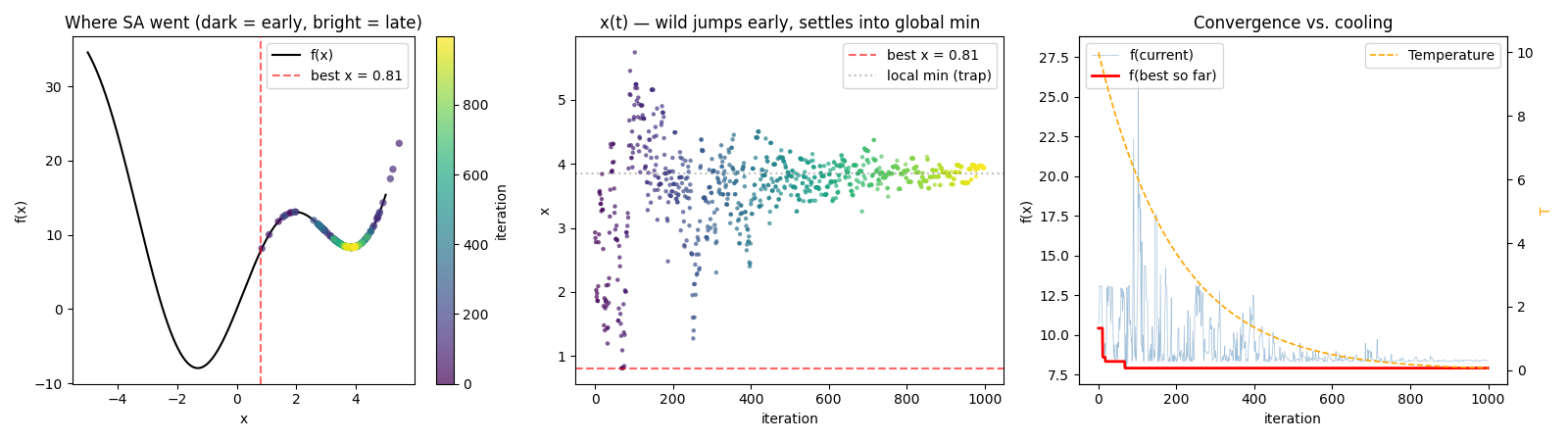
Plot 1 — the “almost made it” trap. T₀ = 10 isn’t enough: SA crosses the peak once (best_x = 0.81 is already past the peak at x ≈ 2 coming from the right!) but T drops faster than x can descend into the global basin. Panel 2 shows it clearly — all 1000 iterations stay between x = 1 and x = 5.

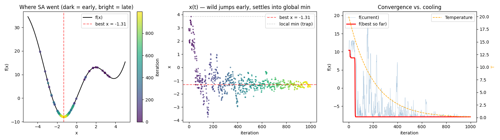
Plot 2 — the clean demo. Doubling the starting temperature (T₀ = 20) gives the algorithm enough “energy budget” to cross the barrier twice — once over, once back, until it settles in the global basin. The Panel 2 dark→bright transition shows the wandering from upper region (x > 0) down to x ≈ −1.31. This is the textbook trajectory.

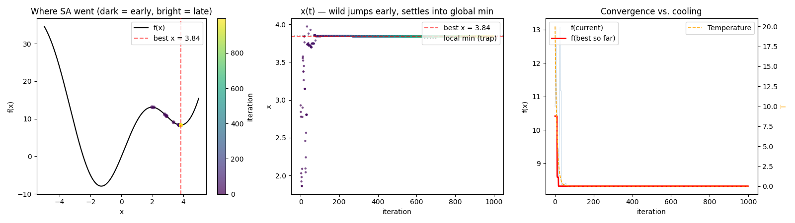
Plot 3 — the most honest failure picture. Look at Panel 3: the orange T-curve drops to ~0 in ~20 iterations. After that, SA = Hill Climbing = stuck in the nearest local min. In Panel 2 you see only a few scattered early purple points between x = 1.5 and 4, then nothing but a flat plateau at x = 3.84. Exactly as predicted.

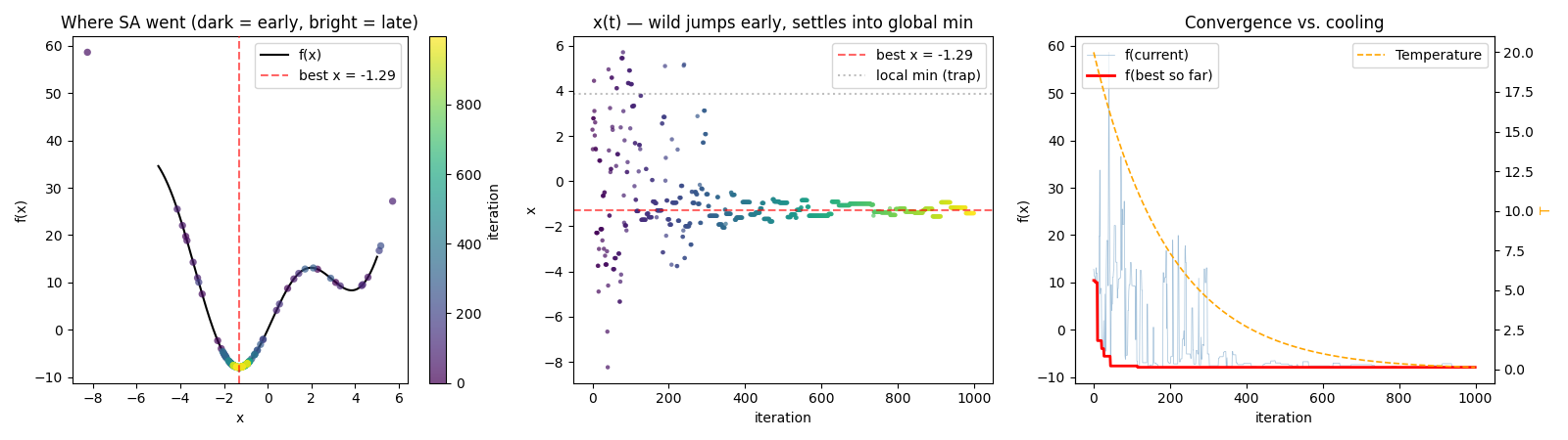
Plot 4 — “success by accident”. Note the outliers at x ≈ −8 (f ≈ 58!) and x ≈ 5.5 — those are single jumps that step = 5 makes possible. The algorithm finds the global min not through gradual climbing, but because a single random move from x = 3 to x ≈ −2 is possible in one step. Panel 2 confirms it: x is scattered across the entire [−8, 6] range, almost no local movement. This is Monte Carlo search, not annealing anymore.

Three takeaways for the exam

T₀ matters. Plot 1 vs. Plot 2: same function, same starting point, same cooling rate — only doubled initial temperature. Success vs. failure.
Cooling matters more than T₀. Plot 3: even with T₀ = 20, cooling = 0.9 is too aggressive. The heat evaporates before it can do work.
Step size distorts the diagnosis. Plot 4 looks like “SA works” — but it doesn’t. If your tests are meant to prove that SA learns to escape, you have to keep step_size small. Otherwise the algorithm dances over the whole landscape and finds the min by random walk.

Bottom line: Plot 2 is the textbook version. The other three each demonstrate one failure mode — and those are exactly the ones to remember for the exam when asked “when does SA fail?”

Where SA is still used today

Despite its age (Kirkpatrick, Gelatt & Vecchi, 1983), SA is still the default tool in many industries where the search landscape is rugged and no gradients exist.

VLSI chip design — the killer application SA was originally invented for. EDA tools (Cadence, Synopsys) still use SA for placement & routing of chips with billions of transistors.
Protein structure prediction — Rosetta@home and similar projects use Monte Carlo with SA-like acceptance to sample protein conformations.
Quantum annealing (D-Wave) — D-Wave’s quantum computers are physical SA: qubit states evolve through a cooling schedule and find the ground state of an Ising Hamiltonian. Volkswagen demonstrated traffic-flow optimization in Beijing with D-Wave (2017); also portfolio optimization and protein folding.
Vehicle routing & logistics — TSP variants for delivery scheduling (UPS, DHL) use SA + restart hybrids.
Medical image registration — aligning CT/MRI scans across patients or time when gradient methods get stuck in local minima.
Compiler optimization — register allocation and instruction scheduling in some compiler backends use SA-style local search.
Hyperparameter tuning — scikit-optimize and some AutoML systems offer SA as an optimizer for high-dimensional search spaces.

Why SA survives: when (a) the objective function is non-differentiable or has many local minima, (b) you can only evaluate but not compute gradients, and (c) you need any reasonable solution quickly — SA is the “no-math-required” baseline that often beats more sophisticated methods.

Where SA was replaced — and by what

Domain	Was SA, now …	Why
Neural network training (early Boltzmann Machines, 1980s)	Backpropagation + SGD (Rumelhart, Hinton 1986)	Once gradients are available, any gradient-based method beats SA by orders of magnitude — the information in the gradient is invaluable
Hyperparameter tuning for ML models	Bayesian Optimization (GPs, TPE) → today often Optuna	BayesOpt uses a probabilistic model of the objective and explores informedly rather than randomly — 10–100× more sample-efficient on expensive evaluations
Pure combinatorial optimization (ILP-shaped)	Gurobi / CPLEX (Branch-and-Cut)	When the problem can be formulated as an Integer Linear Program, commercial MILP solvers with cutting planes + branch-and-bound dominate
Bayesian inference (sampling)	MCMC variants: HMC, NUTS (PyMC, Stan)	SA was historically used as a sampler, but HMC/NUTS use the gradient of the log-posterior and mix far faster
TSP-style problems at small instances	Concorde TSP solver (Branch-and-Cut)	Concorde solves TSPs up to ~85,000 cities optimally — SA only gives approximations

Where SA still stands alone: rugged, non-convex, no gradient, black-box evaluation. Exactly the corner where BayesOpt is too expensive and ILP formulation is impossible.

Brain Online

Explorer

Simulated Annealing