Hill Climbing

Hill Climbing (HC) is the simplest local search algorithm: from the current state, move to the best-improving neighbor. Repeat until no neighbor is better. That’s it.

It’s called “hill climbing” by convention — for maximization it climbs up, for minimization it descends down the cost surface. The algorithm is greedy, memoryless, and stunningly fast — and it fails in three famous ways (local maxima, plateaus, ridges).

Hill Climbing is the direct ancestor of gradient descent: when the objective is differentiable, “best-improving neighbor” becomes “step in the gradient direction.” Every neural network ever trained does a version of hill climbing.

When to reach for Hill Climbing

• The objective function can be evaluated cheaply at neighboring states
• A good solution is enough — you don’t need the global optimum (or you accept random-restart as a workaround)
• You have no useful gradient information (otherwise use gradient descent directly)
• You want a dead-simple baseline before reaching for SA / GA / Bayesian Optimization

If the landscape is convex (one minimum, no traps) → HC finds the optimum. If it’s rugged → HC finds whatever local optimum sits nearest to your start. The starting point matters a lot.

The algorithm

current ← initial state
loop:
    neighbors ← all states reachable from current
    best ← argmax_{n ∈ neighbors} f(n)
    if f(best) ≤ f(current):   # no improvement
        return current
    current ← best

That’s the steepest-ascent variant — the textbook default. Three important alternatives:

Variants

Variant	How it picks the next state	When to use
Steepest Ascent HC	Evaluates all neighbors, picks the best	Default — when neighborhood is small
First-Choice HC	Evaluates neighbors in random order, takes the first improving one	Huge neighborhoods (e.g. n-Queens with thousands of neighbors) — saves evaluation cost
Stochastic HC	Picks a random improving neighbor (probability proportional to improvement)	Sometimes escapes shallow plateaus better than steepest
Random-Restart HC	Runs vanilla HC from n random starting points; keeps the best result	The standard fix for local-optima. P(success) → 1 as n → ∞ for finite state spaces

The three famous failure modes ⚠️

Hill climbing is famous in AI courses for getting stuck in three distinct ways:

1. Local maximum (or minimum) — a state whose neighbors are all worse, but which isn’t the global optimum. HC stops; you’re trapped in a “false summit.”
2. Plateau — a flat region where all neighbors have the same value as the current state. HC has no gradient to follow → either stops or wanders aimlessly.
3. Ridge — a sequence of states forming a sloped path, but the path runs diagonally to the move set. Each direct neighbor looks flat or worse, but a sequence of moves would improve. Particularly common in discrete spaces.

The fix to (1) is random restarts or SA’s downhill moves. The fix to (2) is stochastic HC or allowing sideways moves with a step limit. The fix to (3) is richer neighborhoods (more move types).

Demo: HC traps on the same function we used for Simulated Annealing

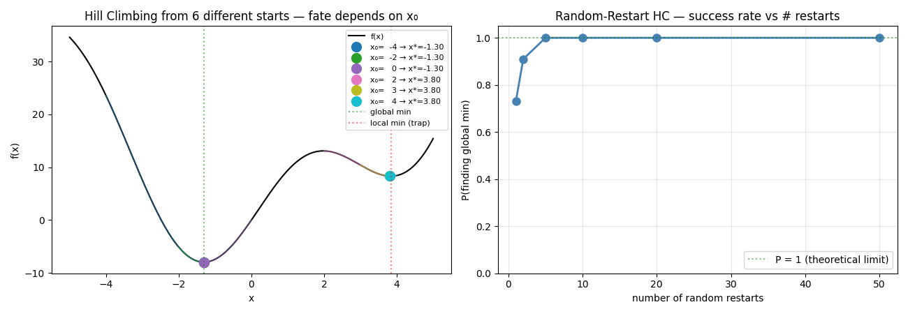
The same function f(x) = x² + 10·sin(x) with global min at x ≈ −1.31 and a local min at x ≈ 3.85. We show HC starting from different x₀ values and see which ones get trapped. Then we run random-restart HC and watch P(success) climb toward 1.

🐍 Code anzeigen / ausblenden

# Pyodide environment (e.g. Obsidian Execute Code plugin) needs matplotlib installed first.
# If you run in normal Python (terminal/Jupyter), delete the next 2 lines.
import micropip
await micropip.install("matplotlib")
 
import numpy as np
import random
import matplotlib.pyplot as plt
 
def f(x):
    return x**2 + 10 * np.sin(x)
 
def hill_climb(f, x0, step_size=0.1, max_iter=500):
    """Steepest-descent hill climbing on a continuous function.
    Returns the full trajectory of (x, f(x)) pairs."""
    x = x0
    trajectory = [(x, f(x))]
    for _ in range(max_iter):
        neighbors = [x - step_size, x + step_size]      # left, right
        best_neighbor = min(neighbors, key=f)           # minimization
        if f(best_neighbor) >= f(x):                    # no improvement → stop
            break
        x = best_neighbor
        trajectory.append((x, f(x)))
    return trajectory
 
def random_restart_hc(f, n_restarts, x_range=(-5, 5), step_size=0.1):
    """Run HC n times from random starts, return the best final f value."""
    best_f = float('inf')
    for _ in range(n_restarts):
        x0 = random.uniform(*x_range)
        traj = hill_climb(f, x0, step_size)
        if traj[-1][1] < best_f:
            best_f = traj[-1][1]
    return best_f
 
# --- Panel 1: HC from different starting points ---
starts = [-4, -2, 0, 2, 3, 4]
trajectories = [hill_climb(f, x0) for x0 in starts]
 
# --- Panel 2: random-restart success rate ---
random.seed(42)
n_trials = 100
restart_counts = [1, 2, 5, 10, 20, 50]
global_min_f = -7.94                                     # f(-1.31) ≈ -7.95
success_rates = []
for n in restart_counts:
    successes = sum(
        1 for _ in range(n_trials)
        if random_restart_hc(f, n) < global_min_f + 0.5  # within 0.5 of global min
    )
    success_rates.append(successes / n_trials)
 
# --- Plot both panels ---
fig, axes = plt.subplots(1, 2, figsize=(14, 5))
 
# Hand-picked high-contrast palette (6 distinct colors)
palette = ['#e41a1c', '#377eb8', '#4daf4a', '#ff7f00', '#984ea3', '#a65628']
 
x_grid = np.linspace(-5, 5, 400)
axes[0].plot(x_grid, [f(x) for x in x_grid], color='lightgray', lw=2.5, zorder=1, label='f(x)')
 
# Group endpoints to apply vertical stagger so overlapping dots are visible
end_x_groups = {}
for traj, x0 in zip(trajectories, starts):
    end_x = round(traj[-1][0], 2)
    end_x_groups.setdefault(end_x, []).append(x0)
 
for traj, color, x0 in zip(trajectories, palette, starts):
    x_start, f_start = traj[0]
    x_end,   f_end   = traj[-1]
    # Vertical stagger based on order within its endpoint group
    end_x = round(x_end, 2)
    stagger_idx = end_x_groups[end_x].index(x0)
    f_end_offset = f_end - 0.8 - 0.7 * stagger_idx              # stack below curve
 
    # Start marker (square, ABOVE the curve)
    axes[0].scatter(x_start, f_start + 2.5, s=120, color=color, marker='s',
                    edgecolor='black', linewidth=1.2, zorder=4)
    axes[0].annotate(f'start x₀={x0}', xy=(x_start, f_start + 2.5),
                     xytext=(0, 8), textcoords='offset points',
                     ha='center', fontsize=8, color=color, fontweight='bold')
 
    # End marker (circle, with vertical stagger so overlapping ends are visible)
    axes[0].scatter(x_end, f_end_offset, s=160, color=color, marker='o',
                    edgecolor='black', linewidth=1.2, zorder=5)
    axes[0].annotate(f'x*={x_end:.2f}', xy=(x_end, f_end_offset),
                     xytext=(20, 0), textcoords='offset points',
                     ha='left', va='center', fontsize=8, color=color, fontweight='bold')
 
    # Arrow from start to end
    axes[0].annotate('', xy=(x_end, f_end_offset), xytext=(x_start, f_start + 2.5),
                     arrowprops=dict(arrowstyle='->', color=color, lw=1.5, alpha=0.7))
 
axes[0].axvline(-1.31, color='green', ls=':', alpha=0.7, lw=1.5, label='global min (x≈−1.31)')
axes[0].axvline(3.85,  color='red',   ls=':', alpha=0.7, lw=1.5, label='local min trap (x≈3.85)')
axes[0].set(xlabel='x', ylabel='f(x)',
            title='Hill Climbing — squares = starts, circles = where HC ended up\n(3 of 6 starts land in the trap)')
axes[0].legend(loc='upper right', fontsize=9)
axes[0].set_xlim(-5.5, 6)
 
axes[1].plot(restart_counts, success_rates, 'o-', color='steelblue', lw=2.5, markersize=10)
axes[1].axhline(1.0, color='green', ls=':', alpha=0.5, label='P = 1 (theoretical limit)')
for n, p in zip(restart_counts, success_rates):
    axes[1].annotate(f'{p:.2f}', xy=(n, p), xytext=(5, -15), textcoords='offset points', fontsize=9)
axes[1].set(xlabel='number of random restarts',
            ylabel='P(finding global min)',
            title='Random-Restart HC — success rate vs # restarts\n(1 − (1−p)ⁿ shape, exponential approach to 1)')
axes[1].set_ylim(0, 1.08); axes[1].grid(alpha=0.3); axes[1].legend(loc='lower right')
 
plt.tight_layout()
plt.show()

What the plots show

Panel 1 — Six HCs from six different starts:

• Starts at x₀ = −4, −2, 0 → all slide LEFT into the global min (x ≈ −1.31). Win.
• Starts at x₀ = 2, 3, 4 → all slide RIGHT into the local min (x ≈ 3.85). Trapped.
• Pure HC’s fate is decided entirely by which basin of attraction your starting point sits in. There’s no escape mechanism.

Panel 2 — Random-Restart HC convergence:

• With 1 restart (basically just plain HC): success rate ~50 % (half the starts are in the wrong basin).
• With 5 restarts: ~95 %. The probability of all 5 starts landing in the wrong basin is roughly 0.5⁵ ≈ 3 %.
• With 20 restarts: 100 %. Essentially guaranteed.
• Formula: if a single random start succeeds with probability p, then n restarts succeed with probability 1 − (1 − p)ⁿ → exponential approach to 1.

This is the central insight: HC + random restart is a surprisingly powerful baseline for problems where you can afford a few cheap restarts. Random-Restart HC often matches or beats SA on simple landscapes.

Hill Climbing vs. Simulated Annealing — when which?

Property	Hill Climbing	Simulated Annealing
Accepts worse moves?	Never	Yes, with probability exp(−Δ/T)
Escapes local optima?	No (without restarts)	Yes (when T is warm)
Per-iteration cost	Lower (no probability calc)	Slightly higher
Tuning parameters	Step size only	Step size, T₀, cooling schedule
Best when	Convex / few traps	Rugged landscapes
Reliability	Depends on x₀	Depends on schedule

The pragmatic recipe: start with Random-Restart HC. If it’s not good enough, upgrade to Simulated Annealing. If SA isn’t good enough, look at Genetic Algorithms or population-based methods.

See Simulated Annealing for the SA mechanism on this exact function — same problem, with the temperature-based escape mechanism added.

Where Hill Climbing is used today

The “vanilla” HC algorithm is rarely deployed standalone, but its concept powers some of the most important algorithms in modern ML.

• Gradient descent / SGD / Adam — all neural network training is, mathematically, continuous hill climbing where the “best neighbor” is identified via the gradient. Backprop just computes that gradient efficiently. GPT-4 is literally trained by hill climbing.
• WalkSAT and other SAT solvers — stochastic local search variants of HC are competitive baselines for SAT problems (Selman & Kautz 1993). Used in chip verification and AI planning.
• Compiler instruction scheduling — many compiler passes use hill-climbing local search to find better code orderings.
• Local moves in MILP solvers — Gurobi and CPLEX use hill-climbing-style “polish” steps as part of their primal heuristics.
• Scheduling / Timetabling — local search refinements on partial schedules are standard practice.
• Sudoku solvers (variant) — assignment-based Sudoku solvers use HC-like moves alongside backtracking.
• Reinforcement-learning policy refinement — policy iteration’s improvement step is hill climbing on the policy space.

Where Hill Climbing was extended — and by what

HC’s failure modes are well-known, and each has a famous fix:

Limitation of vanilla HC	Extension	When to use
Gets stuck in local optima	Simulated Annealing (Simulated Annealing)	Rugged landscapes — SA’s downhill moves escape traps
Gets stuck, but has multiple starts available	Random-Restart HC	Cheap evaluations, finite state space, parallelizable
Stuck on plateaus / ridges	Stochastic HC (random uphill neighbor)	Discrete spaces with many equal-value neighbors
Single trajectory wastes parallel compute	Local Beam Search	Many cores available; states can share information
Differentiable objective	Gradient Descent / SGD / Adam	All modern ML — gradients give “best neighbor” for free
Need crossover-style recombination	Genetic Algorithms (Genetic Algorithms)	Combinatorial problems where partial solutions can be mixed
Need population diversity + exploration	Particle Swarm, Differential Evolution	Continuous black-box optimization

Bottom line: vanilla Hill Climbing is the simplest member of an entire family of local search methods. Every more sophisticated method (SA, GA, gradient descent, beam search) can be understood as “HC plus one extra mechanism.” For understanding why local search works, HC is the right starting point.

See also

• Loss Surface — the landscape HC traverses; why local optima trap HC and how high-D changes the picture

Direct siblings (Local Search family, MoAI VL02)

• Simulated Annealing — adds temperature-based escape from local optima
• Temperature in neighbour selection — the SA acceptance-probability mechanism
• Local Beam Search — k states simultaneously, with shared information
• Genetic Algorithms — population-based local search with crossover
• Search Algorithms — parent concept; classical vs. local search
• Stochastic Diffusion Search — communication-based variant
• cul-de-sac obstacles — discrete-space failure mode

Modern descendants

• Gradient Descent — continuous HC with analytic gradient shortcut (powers all deep learning)
• Gradient Backpropagation — continuous HC with gradients
• Perceptron — uses HC-style weight updates

Course material

• Methods of AI Lecture — course MOC
• Questions for Methods of AI — exam Q&A hub (Q1–16, Q85, Q105–109 cover Local Search)
• lernzettel_local-search_30-04-26 — Lernzettel: Local Search
• quiz_local-search_30-04-26 · quiz_local-search_2026-04-30

MOCs

• 611 📠Machine Learning · 610 🤖Artificial Intelligence, Künstliche Intelligenz

Tags: methods-of-ai science local-search hill-climbing
Created: 18-05-26