SVM: find the hyperplane that maximizes the margin between two classes. Only the support vectors (closest points) determine the hyperplane — all other points have αᵢ = 0.
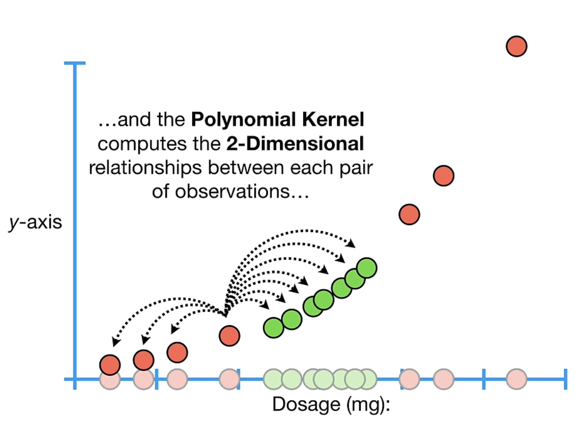
Kernel trick: replace the dot product ⟨x,y⟩ with K(x,y) = ⟨Φ(x),Φ(y)⟩ to classify in higher-dimensional spaces without computing Φ explicitly.
Perceptron: single-layer linear classifier with Heaviside output Θ(s) ∈ {0,1} (NOT sign). Provably convergent if data is linearly separable. Cannot solve XOR.
SVMs handle non-linearity natively via kernels; perceptrons need multi-layer extension (MLP) for non-linear tasks.
Glossary — important SVM/Perceptron vocabulary ⭐
Hyperplane H — an (n−1)-dimensional separating surface in Rⁿ, defined by H = {x ∈ Rⁿ | ⟨w,x⟩ + b = 0}.
Example: in R² a hyperplane is a line; in R³ it’s a plane.
Weight vector w ∈ Rⁿ — vector orthogonal to the hyperplane. Determines orientation; its magnitude ‖w‖ inversely sets the margin width.
Bias b ∈ R — offset of the hyperplane from the origin along w. (In the perceptron, the bias is absorbed as w₀ by prepending a constant input x₀ = 1.)
Margin — distance between the two parallel “support” hyperplanes ⟨w,x⟩+b = +1 and ⟨w,x⟩+b = −1. Equals 2/‖w‖. SVM maximizes this.
Support vector — a training point that lies exactly on one of the two margin hyperplanes. Only these points have αᵢ > 0. They alone determine w.
Visual cue: in a 2D drawing, the support vectors are the points that “touch” the margin lines.
Lagrange multiplier αᵢ ≥ 0 — one per training point. αᵢ > 0 ⇔ point i is a support vector. From the KKT condition αᵢ · (yᵢ(⟨xᵢ,w⟩+b) − 1) = 0.
Kernel K(x,y) — a function K: X × X → R such that there exists a mapping Φ: X → H with K(x,y) = ⟨Φ(x), Φ(y)⟩. Lets us compute dot products in feature space without ever computing Φ.
RBF (Radial Basis Function) — the Gaussian kernel K(x,y) = exp(−‖x−y‖²/2σ²). “Radial” = depends only on the distance ‖x−y‖; “basis function” = each SV is a localized bump. Maps into an infinite-dim feature space. σ (or γ = 1/2σ²) sets bump width.
PSD (Positive Semi-Definite)(suppl.) — property of the kernel/Gram matrix K: cᵀKc ≥ 0 for all c (all eigenvalues ≥ 0). Mercer: K PSD ⟺ ∃ φ with K(x,y)=⟨φ(x),φ(y)⟩, and it keeps the SVM dual convex.
Slack variable ξᵢ ≥ 0 (soft-margin, supplementary) — how much constraint i is allowed to be violated. ξᵢ = 0 → no violation; 0 < ξᵢ < 1 → inside margin but correctly classified; ξᵢ ≥ 1 → misclassified.
C parameter(soft-margin, supplementary) — trade-off knob between margin size and number of violations. Large C → small tolerance for misclassification (narrow margin, overfitting risk); small C → large margin, more violations allowed (more regularization).
Heaviside step Θ(s) — perceptron output activation: Θ(s) = 1 if s ≥ 0, else 0. (NOT sign(s) ∈ {−1,+1}.)
Preactivation s = w·x = w₀·1 + w₁x₁ + … + w_d x_d — the linear combination before applying Θ. The “gradient” in perceptron training is taken w.r.t. this preactivation (slide 44).
Linear separability — the property that two classes can be separated by a hyperplane. Necessary condition for perceptron convergence.
SVM — Maximum Margin Classifier
Setup
Training data: pairs (x₁,y₁), …, (x_N,y_N) with xᵢ ∈ Rⁿ and yᵢ ∈ {+1, −1}.
Find f: Rⁿ → {+1, −1} with f(xᵢ) = yᵢ on training data; classify unseen x via f(x).
Hyperplane
A separating affine hyperplane:
H = {x ∈ Rⁿ | ⟨w, x⟩ + b = 0}
with w ∈ Rⁿ orthogonal to H, b ∈ R.
⟨w, x⟩ + b > 0 → positive class
⟨w, x⟩ + b < 0 → negative class
⟨w, x⟩ + b = 0 → on the hyperplane
Two parallel margin hyperplanes
We canonicalize by demanding:
⟨w, x₁⟩ + b = +1 (closest positive point)
⟨w, x₂⟩ + b = −1 (closest negative point)
Maximizing the αᵢ while minimizing w and b (saddle-point problem) yields:
w = Σᵢ αᵢ · yᵢ · xᵢ
⇒ The weight vector is a linear combination of the training examples, weighted by αᵢ·yᵢ.
Karush-Kuhn-Tucker (KKT) saddle-point condition
αᵢ · (yᵢ · (⟨xᵢ, w⟩ + b) − 1) = 0 for all i
⇒ For each i, either αᵢ = 0 or yᵢ(⟨xᵢ,w⟩+b) = 1 (point lies exactly on the margin).
αᵢ > 0 ⇒ point i is a support vector (on the margin)
αᵢ = 0 ⇒ point i is interior to its side; does not influence w at all
Hence:
w = Σᵢ : xᵢ is support vector αᵢ · yᵢ · xᵢ
How are support vectors chosen?
⭐ They are not chosen — they fall out of the optimization. There is no selection heuristic; the QP solver assigns every point an αᵢ, and the support vectors are simply the points whose margin constraint ends up active (tight). The KKT complementary-slackness condition above forces exactly one of two cases per point:
Point’s situation
Constraint yᵢ(⟨xᵢ,w⟩+b)
Multiplier
Support vector?
strictly outside the margin (correct, far away)
> 1 (slack)
αᵢ = 0
No
exactly on the margin boundary
= 1 (tight/active)
αᵢ > 0
Yes
A far-away point has a non-tight constraint, so the only way to satisfy αᵢ·(…−1)=0 is αᵢ = 0 → it drops out. Only points on the margin can carry αᵢ > 0.
Consequences (exam-favourites):
The hyperplane depends only on the support vectors. Delete every non-SV and retrain → identical boundary.
Move/remove a support vector → the boundary changes. They “hold the margin in place.”
This is SVM sparsity: typically few SVs, so prediction sums over them only.
Soft-margin: support vectors come in two flavours (suppl., C/slack — not in Session 11 slides)
With slack ξᵢ and the box bound 0 ≤ αᵢ ≤ C:
0 < αᵢ < C → point lies exactly on the margin.
αᵢ = C → point violates the margin (inside it or misclassified).
⚠️ Trap: “support vectors = the closest points” is only loosely true. Precisely, they are the points with active constraints (αᵢ > 0) — on the margin (hard case) or violating it (soft case). It’s the optimization, not a distance ranking, that picks them out.
Decision function
For a new input x:
f(x) = sgn(Σᵢ αᵢ · yᵢ · ⟨x, xᵢ⟩ + b)
The sum runs over training points; only support vectors actually contribute (the rest have αᵢ = 0). The decision uses only dot products ⟨x, xᵢ⟩ — which sets up the kernel trick.
Kernel Trick
Replace every dot product in the decision function with a kernel K:
f(x) = sgn(Σᵢ αᵢ · yᵢ · K(x, xᵢ) + b)
where K(x, x′) = ⟨Φ(x), Φ(x′)⟩ for some mapping Φ: X → H to a (possibly very high-dim) feature space H.
Why this is powerful. Φ may map to a 10⁶-dimensional or even infinite-dimensional space, but K(x,x′) is computed in the original input space — typically in O(n) operations. We never have to actually compute Φ(x).
Key requirement. K must correspond to an inner product in some Hilbert space. The textbook (R&N) calls this Mercer’s condition — not in Session 11 slides; supplementary.
PSD-ness — why the kernel trick is legal (suppl., tied to Mercer)
Mercer’s condition makes precise what “K is a valid kernel” means: the Gram matrix K (with Kᵢⱼ = K(xᵢ, xⱼ) over any finite set of inputs) must be positive semi-definite (PSD):
cᵀ K c ≥ 0 for all vectors c ⟺ all eigenvalues of K are ≥ 0
This buys two things:
A feature map is guaranteed to exist. PSD ⟺ there is some φ with K(x, y) = ⟨φ(x), φ(y)⟩. So you can treat K as an honest dot product in feature space without ever building φ — exactly the kernel trick.
The dual QP stays convex. The dual objective W(α) = Σαᵢ − ½ ΣᵢΣⱼ αᵢαⱼ yᵢyⱼ K(xᵢ,xⱼ) has the kernel matrix as its quadratic form. PSD ⇒ concave maximization ⇒ one global optimum, reliably solvable. A non-PSD kernel makes the objective non-convex → local optima → the QP solver can return garbage.
⚠️ Exam traps: (i) it’s semi-definite — eigenvalues ≥ 0, not strictly > 0; (ii) it’s the Gram matrix that must be PSD, not the raw data; (iii) symmetry alone is not enough — symmetric + PSD is the full condition.
🔗 Full deep dive with worked polynomial-kernel verification, RBF visualisation, and Mercer details: see Kernel Trick.
Common Kernels
Kernel
Formula
Hyper-parameters
Linear
K(x, y) = ⟨x, y⟩
—
Polynomial
K(x, y) = (⟨x, y⟩ + c)^d
c ≥ 0, degree d ∈ ℕ
RBF / Gaussian
K(x, y) = exp(−‖x − y‖² / 2σ²)
σ > 0 (width)
RBF = Radial Basis Function. “Radial” → the kernel depends only on the distance ‖x−y‖ (a radius), not on direction or absolute position; “basis function” → each support vector acts as a localized bump, and the decision function is a weighted sum of these bumps. It implicitly maps into an infinite-dimensional feature space, which is why it can separate almost any dataset.
⚠️ Notation: many sources write the RBF kernel as exp(−γ · ‖x−y‖²) with γ = 1/(2σ²). The two are equivalent; the Session 11 slide uses the σ-form (the γ-form appears later only for the soft tree kernel). σ (or γ) controls the bump width: small σ / large γ → narrow bumps → overfitting; large σ / small γ → smooth, near-linear boundary.
Not covered in Session 11 slides — from R&N textbook background. May appear in oral exams.
Real data is rarely perfectly linearly separable. Soft-margin SVM relaxes the hard constraint by introducing slack variables ξᵢ ≥ 0:
minimize ½‖w‖² + C · Σᵢ ξᵢ
subject to yᵢ(⟨xᵢ, w⟩ + b) ≥ 1 − ξᵢ, ξᵢ ≥ 0
ξᵢ = 0 → point i is on the correct side of the margin (good).
0 < ξᵢ < 1 → inside the margin but still correctly classified.
ξᵢ ≥ 1 → misclassified.
C parameter controls the trade-off:
Large C → heavy penalty on slack → small margin, few violations → risk of overfitting.
Small C → cheap slack → large margin, more violations allowed → more regularization.
C = ∞ recovers the hard-margin SVM; C = 0 makes the algorithm ignore the data entirely.
Perceptron
🔗 Full atomic note with biological-neuron motivation, AND/XOR Python demo, and history of where perceptrons are used today: see Perceptron.
Architecture (slide 36–37)
For an input x ∈ Rᵈ:
Preactivation: s = w₀ + w₁x₁ + w₂x₂ + … + w_d x_d Output (activation): y = Θ(s) = 1 if s ≥ 0, else 0
w₀ acts as a threshold. To unify notation, we prepend a constant input x₀ = 1:
x = (1, x₁, …, x_d)ᵀ ∈ R^(d+1)
w = (w₀, w₁, …, w_d)ᵀ ∈ R^(d+1)
s = x · w, y = Θ(x · w)
⚠️ Slide convention: the perceptron output is Θ ∈ {0, 1} (Heaviside), NOT sign(·) ∈ {−1, +1}. Many textbooks use the sign-version; the slide deck (and the exam) uses Heaviside.
Decision surface (slide 38)
Perceptron represents the hypothesis space {w | w ∈ R^(d+1)}. The decision surface is the (d−1)-dim hyperplane orthogonal to w. Points with x·w > 0 get y = 1; the rest y = 0.
Class separability (slide 39)
A perceptron can solve a classification task only if the two classes are linearly separable — separable by some hyperplane.
Training rule (derivation, slides 43–45)
The learning rule is derived from minimizing the mean square error (MSE):
E[w; D] = ½ · Σₙ (tⁿ − y(xⁿ))²
with tⁿ ∈ {0, 1} the target label.
⚠️ Why this is “gradient descent in scare quotes”: the activation Θ is not differentiable at 0 and has zero gradient elsewhere — so true gradient descent is impossible. Slide 44 sidesteps this by taking the gradient w.r.t. the preactivation w·x (i.e., treating y(x) as if it were w·x for the gradient step). The result is the standard perceptron update rule.
For small enough ε, stochastic gradient descent approximates batch arbitrarily closely.
XOR problem
The problem (slide 41)
A 2-input perceptron with constant bias can implement AND, OR, NAND, NOR — but not XOR. XOR’s positive examples ((0,1) and (1,0)) and negative examples ((0,0) and (1,1)) are not linearly separable in R².
The fix (slide 42)
Nonlinear feature mapping: transform input x via some f(x) into a feature space where XOR is linearly separable.
Add an extra input channel: e.g. x₃ = x₁ · x₂. Now the 3D representation is linearly separable.
This is the same idea SVMs formalize as the kernel trick.
Historical consequence (slide 47, exact wording)
The fact that perceptrons cannot solve XOR “led to a temporary drop in the interest in ANN”.
⚠️ The dramatic phrasing “AI winter” and the famous Minsky & Papert (1969) book are textbook background, not present in the slide deck. The slides only say “temporary drop in interest”.
Only support vectors matter. Non-support-vector training points have αᵢ = 0 and contribute nothing to w. This is the core insight of SVMs.
Lagrangian sign convention. The standard SVM Lagrangian uses a minus sign in front of the αᵢ-term (because the constraint is yᵢ(⟨xᵢ,w⟩+b) − 1 ≥ 0 and we subtract the constraint × multiplier for a minimization). Getting this sign wrong flips the saddle-point direction.
Margin = 2/‖w‖, NOT 1/‖w‖. The factor 2 comes from the distance between the two parallel margin hyperplanes (+1 and −1 sides).
Large C ≠ better. Large C prioritizes correct classification over a large margin → overfitting risk. (Supplementary — not in slides.)
Kernel trick ≠ explicit mapping. The kernel computes the dot product in feature space without ever evaluating Φ. This makes infinite-dim feature spaces (RBF) tractable.
SVM maximizes margin, not training accuracy. A wider-margin solution can be preferred even if a narrower one classifies all training points correctly.
Perceptron convergence theorem is conditional. Guaranteed ONLY if data is linearly separable. If not, it never converges.
Perceptron output is Θ(s) ∈ {0,1}, not sign(s) ∈ {−1,+1}. Be careful when reading textbook problems that use the sign-version.
Bias in perceptron is absorbed. w₀ is just another weight, with a constant input x₀ = 1. No separate update rule.
“Gradient” descent on perceptron MSE is misleading. Θ is not differentiable. Slide 44 takes the gradient w.r.t. the preactivation w·x, not the output y.
XOR → “temporary drop in interest in ANN” (slide 47 wording). “AI winter” and “Minsky & Papert” are textbook embellishments.
PSD-ness ≠ PD. A valid kernel needs a positive semi-definite Gram matrix (eigenvalues ≥ 0, zeros allowed) — not strictly positive-definite. PSD is what guarantees both the feature map φ and dual convexity; a non-PSD “kernel” breaks the convex QP. (Supplementary — tied to Mercer.)
Mercer’s condition, PSD-ness, soft-margin SVM, slack variables, C parameter are NOT in Session 11 slides — supplementary R&N material.
Visualisations (Python)
Figures that bring the math to life. Render each toggle, then read the explanation underneath.
🐍 Demo — how support vectors are chosen (real sklearn fit, not hand-picked)
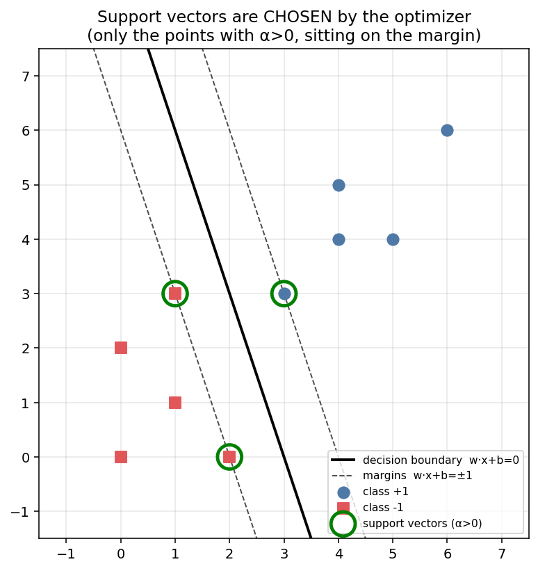
The point of this one: we don’t pick the support vectors — the optimizer does. We fit a real linear SVM, then check y·f(x) for every training point. The support vectors are exactly the points the solver gave α > 0, and those are exactly the points sitting on the margin (y·f(x) = 1). See How are support vectors chosen?.
import numpy as npfrom sklearn.svm import SVC# small, linearly separable 2D dataset (labels +1 / -1)X = np.array([[3,3],[4,5],[5,4],[6,6],[4,4], # positive class [1,1],[2,0],[0,2],[1,3],[0,0]]) # negative classy = np.array([1,1,1,1,1, -1,-1,-1,-1,-1])clf = SVC(kernel="linear", C=1e6) # large C -> hard-margin behaviourclf.fit(X, y)w, b = clf.coef_[0], clf.intercept_[0]f = X @ w + b # decision value f(x) = w·x + bmargin = y * f # y·f(x): == 1 ON the margin, > 1 if interiorsv = set(clf.support_.tolist()) # indices the optimizer flagged as SVs (α>0)for i,(xi,yi,fi,mi) in enumerate(zip(X,y,f,margin)): print(f"{str(tuple(xi)):>7} y={yi:+d} f(x)={fi:6.2f} y·f(x)={mi:5.2f}" f"{' <-- alpha>0 SUPPORT VECTOR' if i in sv else ''}")
Read it: every point with y·f(x) = 1.00 (the active/tight constraint) is a support vector; every point with y·f(x) > 1 (slack) is interior and gets α = 0. The optimizer chose 3 support vectors — (3,3), (2,0), (1,3) — purely from the constraints, no distance ranking. clf.dual_coef_ holds their αᵢ·yᵢ; w = Σ αᵢ yᵢ xᵢ uses only these three. (Runs locally with scikit-learn; sklearn isn’t reliably available in the in-note Pyodide runner, so the verified output + figure are embedded.)
The three circled points are the support vectors the optimizer selected — note they all lie exactly on the dashed margin lines, while every other point is strictly past its margin (and thus irrelevant to w).
🐍 Figure — 2D linear SVM with max margin and support vectors
import micropipawait micropip.install("matplotlib")import matplotlib.pyplot as pltimport numpy as np# Toy 2D dataset — linearly separable, hand-picked so support vectors are obvious.# Positive class (y=+1) and negative class (y=-1).X_pos = np.array([[3, 3], [4, 5], [5, 4], [6, 6], [4, 4]])X_neg = np.array([[1, 1], [2, 0], [0, 2], [1, 3], [0, 0]])# By inspection the closest pair across classes is (3,3) [pos] and (1,1) [neg].# The max-margin hyperplane is perpendicular to (3,3)-(1,1) = (2,2), so w ∝ (1,1).# Canonicalise w so that y·(w·x + b) = 1 for support vectors:# (3,3): w·x + b = +1 → 3w1 + 3w2 + b = +1# (1,1): w·x + b = -1 → w1 + w2 + b = -1# With w = (a, a): 6a + b = 1, 2a + b = -1 → 4a = 2 → a = 0.5, b = -2.w = np.array([0.5, 0.5])b = -2.0support_vectors = np.array([[3, 3], [1, 1]])# Plotfig, ax = plt.subplots(figsize=(8, 7))# Decision boundary: w·x + b = 0 → x2 = -(w1·x1 + b)/w2xs = np.linspace(-1, 7, 100)ys_boundary = -(w[0] * xs + b) / w[1]ys_pos_margin = -(w[0] * xs + b - 1) / w[1] # w·x + b = +1ys_neg_margin = -(w[0] * xs + b + 1) / w[1] # w·x + b = -1ax.plot(xs, ys_boundary, "k-", lw=2, label="decision boundary w·x+b=0")ax.plot(xs, ys_pos_margin, "k--", lw=1.2, alpha=0.7, label="margin w·x+b=±1")ax.plot(xs, ys_neg_margin, "k--", lw=1.2, alpha=0.7)# Shade the margin bandax.fill_between(xs, ys_neg_margin, ys_pos_margin, color="gray", alpha=0.12)# Data pointsax.scatter(X_pos[:, 0], X_pos[:, 1], c="#e74c3c", s=110, edgecolor="black", lw=1.2, label="class +1", zorder=3)ax.scatter(X_neg[:, 0], X_neg[:, 1], c="#3498db", s=110, edgecolor="black", lw=1.2, label="class −1", zorder=3)# Circle the support vectorsax.scatter(support_vectors[:, 0], support_vectors[:, 1], s=320, facecolors="none", edgecolors="#27ae60", lw=2.5, label="support vectors (α>0)", zorder=4)margin_width = 2 / np.linalg.norm(w)ax.set_title(f"2D linear SVM — max-margin classifier\n" f"w = (0.5, 0.5), b = -2 → margin = 2/‖w‖ = {margin_width:.3f}", fontsize=11)ax.set_xlabel("x₁"); ax.set_ylabel("x₂")ax.set_xlim(-1, 7); ax.set_ylim(-1, 7)ax.legend(loc="lower right", fontsize=9, framealpha=0.95)ax.set_aspect("equal"); ax.grid(alpha=0.3)plt.tight_layout(); plt.show()
What this shows. A toy 2D dataset with 5 positive (red) and 5 negative (blue) points. The solid line is the SVM decision boundary; the dashed lines are the two parallel margin hyperplanes w·x+b = ±1. The two support vectors circled in green — (3,3) and (1,1) — are the only points that touch the margin. Every other point sits strictly inside its own half-plane and contributes αᵢ = 0 to the solution. If you deleted any non-circled point and re-trained, the hyperplane would be unchanged. That is what “only support vectors matter” looks like geometrically. Margin width = 2/‖w‖ = 2√2 ≈ 2.83.
What this shows. Two concentric rings in R² (left) are the classic non-linearly-separable dataset — no straight line can split inner from outer. Apply the mapping φ(x₁, x₂) = (x₁, x₂, x₁² + x₂²): the new third coordinate is the squared radius, which is small (~1) for the inner ring and large (~6.25) for the outer one. In the lifted 3D space (right), a horizontal plane at z ≈ 3 perfectly separates the classes — i.e. the problem is now linear. This is the kernel trick in action: instead of computing φ explicitly, an SVM with a polynomial kernel K(x,y) = (⟨x,y⟩+1)² evaluates the inner product in this lifted space directly in O(d) input-space ops.
🐍 Figure — Perceptron learning trace (OR gate)
import micropipawait micropip.install("matplotlib")import matplotlib.pyplot as pltimport numpy as np# OR-gate dataset — linearly separable, 2D# Input (x1, x2), with absorbed bias x0=1 → x̃ = (1, x1, x2)X = np.array([[1, 0, 0], [1, 0, 1], [1, 1, 0], [1, 1, 1]])t = np.array([0, 1, 1, 1])def heaviside(s): return (s >= 0).astype(int)def train(epochs_to_record, lr=1.0, seed=0): rng = np.random.default_rng(seed) w = np.zeros(3) snapshots = {} max_epoch = max(epochs_to_record) for ep in range(1, max_epoch + 1): order = rng.permutation(len(X)) for i in order: y = heaviside(w @ X[i]) w = w + lr * (t[i] - y) * X[i] if ep in epochs_to_record: snapshots[ep] = w.copy() return snapshotssnaps = train(epochs_to_record=[1, 3, 10], lr=1.0, seed=0)fig, axes = plt.subplots(1, 3, figsize=(15, 5))for ax, (ep, w) in zip(axes, snaps.items()): # Plot data for xi, ti in zip(X[:, 1:], t): color = "#e74c3c" if ti == 1 else "#3498db" ax.scatter(xi[0], xi[1], c=color, s=220, edgecolor="black", lw=1.5, zorder=3) ax.text(xi[0], xi[1] + 0.12, f"t={ti}", ha="center", fontsize=9) # Decision boundary: w0 + w1·x1 + w2·x2 = 0 xs = np.linspace(-0.4, 1.4, 100) if abs(w[2]) > 1e-9: ys = -(w[0] + w[1] * xs) / w[2] ax.plot(xs, ys, "k-", lw=2, label=f"w = ({w[0]:.1f}, {w[1]:.1f}, {w[2]:.1f})") elif abs(w[1]) > 1e-9: x_vert = -w[0] / w[1] ax.axvline(x_vert, color="k", lw=2, label=f"w = ({w[0]:.1f}, {w[1]:.1f}, {w[2]:.1f})") else: ax.text(0.5, 0.5, "w = 0 → no boundary", ha="center", transform=ax.transAxes, fontsize=11) # Shade y=1 region (s = w·x ≥ 0) xx, yy = np.meshgrid(np.linspace(-0.4, 1.4, 80), np.linspace(-0.4, 1.4, 80)) s = w[0] + w[1] * xx + w[2] * yy ax.contourf(xx, yy, s, levels=[0, 1e9], colors=["#e74c3c"], alpha=0.12) ax.set_title(f"Epoch {ep}", fontsize=12) ax.set_xlabel("x₁"); ax.set_ylabel("x₂") ax.set_xlim(-0.4, 1.4); ax.set_ylim(-0.4, 1.4) ax.set_aspect("equal"); ax.grid(alpha=0.3) ax.legend(loc="lower right", fontsize=9, framealpha=0.95)fig.suptitle("Perceptron training trace — OR gate (ε=1, stochastic, " "Heaviside output)", fontsize=12, fontweight="bold")plt.tight_layout(); plt.show()
What this shows. Three snapshots of the perceptron’s decision boundary while training on the OR gate. After epoch 1 the weights have barely separated anything; by epoch 3 the boundary is sweeping into a usable region; by epoch 10 the perceptron has converged to a valid OR-separating line (the red-shaded region covers exactly the three positive points (0,1), (1,0), (1,1) while leaving (0,0) on the y=0 side). Convergence is guaranteed because OR is linearly separable — that is the Perceptron Convergence Theorem. Try changing the dataset to XOR and the boundary will oscillate forever, since no straight line works.
🐍 Figure — Soft-margin C parameter effect ⚠️ supplementary
What this shows.Supplementary — soft-margin is NOT in Session 11 slides. The same partially-overlapping 2D dataset trained with three values of C. Left (C=0.1): large penalty on ‖w‖, low penalty on violations → wide margin, many points lie inside it (these become bounded support vectors with αᵢ = C). Middle (C=1): balanced. Right (C=100): algorithm strongly insists on correct classification → narrow margin, fewer SVs, potential overfit. As C → ∞ you recover the hard-margin SVM; as C → 0 the algorithm ignores the data. This is the canonical bias-variance knob for SVMs.
ALGORITHMS (full reference) ⭐
1. Perceptron training (online + batch) ⭐
Goal. Iteratively update w to classify all training points correctly (if possible).
Online (stochastic) mode
PERCEPTRON-ONLINE(D, ε, max_epochs):
    w ← 0   # or small random
    for epoch in 1..max_epochs:
        any_update ← false
        for each (xⁿ, tⁿ) in shuffle(D):
            xⁿ ← prepend(1, xⁿ)              # absorb bias as x₀ = 1
            yⁿ ← Θ(w · xⁿ)                   # Heaviside ∈ {0, 1}
            if yⁿ ≠ tⁿ:
                Δw ← ε · (tⁿ − yⁿ) · xⁿ
                w ← w + Δw
                any_update ← true
        if not any_update: return w            # converged
    return w
Batch mode
PERCEPTRON-BATCH(D, ε, max_epochs):
    w ← 0
    for epoch in 1..max_epochs:
        gradient ← 0
        for each (xⁿ, tⁿ) in D:
            xⁿ ← prepend(1, xⁿ)
            yⁿ ← Θ(w · xⁿ)
            gradient ← gradient + (tⁿ − yⁿ) · xⁿ
        Δw ← ε · gradient
        if ‖Δw‖ < tol: return w
        w ← w + Δw
    return w
Convergence. Guaranteed iff (i) the data is linearly separable, (ii) ε is small enough. Update rule per example. Δw = ε · (tⁿ − yⁿ) · xⁿ — equals 0 when the prediction is already correct (so correctly-classified points stop influencing w). Cost per epoch. O(|D| · (d+1)).
2. SVM constrained QP optimization (conceptual) ⭐
Goal. Solve the primal problem
min ½‖w‖² s.t. yᵢ(⟨xᵢ,w⟩+b) ≥ 1 for all i.
SVM-TRAIN(D = {(xᵢ, yᵢ)}):
    # Step 1: build the Lagrangian
    L(w, b, α) = ½‖w‖² − Σᵢ αᵢ · (yᵢ(⟨xᵢ,w⟩+b) − 1)
                 with αᵢ ≥ 0

    # Step 2: stationarity conditions
    ∂L/∂w = w − Σᵢ αᵢ yᵢ xᵢ = 0   ⇒   w = Σᵢ αᵢ yᵢ xᵢ
    ∂L/∂b = −Σᵢ αᵢ yᵢ = 0          ⇒   Σᵢ αᵢ yᵢ = 0

    # Step 3: substitute → dual problem (only αᵢ left)
    maximize  W(α) = Σᵢ αᵢ − ½ Σᵢ Σⱼ αᵢ αⱼ yᵢ yⱼ ⟨xᵢ, xⱼ⟩
    subject to  αᵢ ≥ 0,  Σᵢ αᵢ yᵢ = 0

    # Step 4: solve the dual (convex QP) with any QP solver
    α* ← QP-SOLVE(dual)

    # Step 5: recover w and b
    w  ← Σᵢ α*ᵢ yᵢ xᵢ
    SV ← { i | α*ᵢ > 0 }                     # support vectors
    b  ← yₛ − ⟨w, xₛ⟩  for any s ∈ SV         # (average over all SVs in practice)
    return (w, b, α*, SV)
Key takeaway. The QP is convex → unique global optimum. The decision function depends only on dot products ⟨xᵢ, xⱼ⟩ — which is exactly where kernels plug in (just replace ⟨xᵢ, xⱼ⟩ with K(xᵢ, xⱼ)).
3. Kernel evaluation
Goal. Compute K(x, x′) = ⟨Φ(x), Φ(x′)⟩ without ever building Φ.
KERNEL-EVAL(x, x', type, params):
    if type == "linear":
        return dot(x, x')

    if type == "polynomial":         # K(x,y) = (⟨x,y⟩ + c)^d
        c, d ← params
        return (dot(x, x') + c) ** d

    if type == "rbf":                # K(x,y) = exp(−‖x−y‖² / 2σ²)
        σ ← params
        return exp(−norm(x − x')**2 / (2 * σ**2))
Classification with kernels.
SVM-CLASSIFY(x, SV, α, y, b, K):
    s ← b
    for each i in SV:
        s ← s + αᵢ · yᵢ · K(x, xᵢ)
    return sgn(s)
Cost per prediction. O(|SV| · n) — does not depend on the (possibly infinite) feature-space dimension.
4. Soft-margin SVM extension (supplementary)
Not in Session 11 slides — R&N textbook material.
SVM-SOFT(D, C):
    # Primal:
    minimize ½‖w‖² + C · Σᵢ ξᵢ
    subject to yᵢ(⟨xᵢ,w⟩+b) ≥ 1 − ξᵢ,  ξᵢ ≥ 0

    # Dual (the only thing that changes vs. hard-margin):
    maximize  W(α) = Σᵢ αᵢ − ½ Σᵢ Σⱼ αᵢ αⱼ yᵢ yⱼ K(xᵢ, xⱼ)
    subject to  0 ≤ αᵢ ≤ C,   Σᵢ αᵢ yᵢ = 0

    α* ← QP-SOLVE(dual)
    # same w, b, classification as hard-margin
Effect of C. The single change vs. hard-margin: αᵢ is now bounded above by C. Points with αᵢ = C are “bound” support vectors lying inside or beyond the margin. Smaller C ⇒ more bounded SVs ⇒ wider margin ⇒ more regularization.
Worked examples
SVM 2D worked example — identify support vectors
Setup. 4 training points in R²:
Positive class (y = +1): (3, 3), (4, 5)
Negative class (y = −1): (1, 1), (2, 0)
Eyeballing, the two classes are separated by a line roughly running NW–SE between them. The maximum-margin separator is the line equidistant from the closest positive and closest negative point.
Step 1 — find closest pairs.
(3,3)+ is the closest positive to the negatives.
(1,1)− is the closest negative to (3,3)+.
The midpoint of (3,3) and (1,1) is (2, 2), and the line normal to (3,3)−(1,1) = (2, 2) through (2, 2) is the candidate separator: x₁ + x₂ = 4.
So the two non-support points (4,5) and (2,0) are interior to their sides — they get αᵢ = 0 and have no influence on w. The support vectors are exactly (3, 3) and (1, 1) — αᵢ > 0 for these two only.
Step 3 — read off w and margin.
Direction of w: (3,3) − (1,1) = (2, 2), normalized: (1/√2, 1/√2). The SVM solution scales w so that the two SVs sit exactly on the ±1 hyperplanes.
Punchline. If you removed (4,5) or (2,0) and re-ran the SVM, the answer would be identical. If you removed (3,3) or (1,1), the entire hyperplane would shift. That is what “only support vectors matter” means in practice.
Perceptron training trace
Setup. Learn the AND function with 2 inputs (Heaviside output, slide convention).
Training data (with absorbed bias x₀ = 1):
n
xⁿ = (1, x₁, x₂)
tⁿ
1
(1, 0, 0)
0
2
(1, 0, 1)
0
3
(1, 1, 0)
0
4
(1, 1, 1)
1
Initialize w = (0, 0, 0), ε = 1, stochastic mode.
Epoch 1:
step
xⁿ
s = w·x
y = Θ(s)
tⁿ
(t−y)
Δw = ε(t−y)xⁿ
new w
1
(1,0,0)
0
1
0
−1
(−1, 0, 0)
(−1, 0, 0)
2
(1,0,1)
−1
0
0
0
(0, 0, 0)
(−1, 0, 0)
3
(1,1,0)
−1
0
0
0
(0, 0, 0)
(−1, 0, 0)
4
(1,1,1)
−1
0
1
+1
(+1, +1, +1)
(0, 1, 1)
Epoch 2:
step
xⁿ
s
y
t
(t−y)
Δw
new w
1
(1,0,0)
0
1
0
−1
(−1,0,0)
(−1, 1, 1)
2
(1,0,1)
0
1
0
−1
(−1,0,−1)
(−2, 1, 0)
3
(1,1,0)
−1
0
0
0
(0,0,0)
(−2, 1, 0)
4
(1,1,1)
−1
0
1
+1
(+1,+1,+1)
(−1, 2, 1)
Epoch 3 (check): with w = (−1, 2, 1):
(1,0,0): s = −1, y = 0 ✓
(1,0,1): s = 0, y = 1 ✗ ⇒ update Δw = (−1, 0, −1) ⇒ w = (−2, 2, 0)
(1,1,0): s = 0, y = 1 ✗ ⇒ update Δw = (−1, −1, 0) ⇒ w = (−3, 1, 0)
(1,1,1): s = −2, y = 0 ✗ ⇒ update Δw = (+1, +1, +1) ⇒ w = (−2, 2, 1)
Training continues; a valid AND-separating w exists (e.g. w = (−3, 2, 2): check (1,0,0)→s=−3→0, (1,0,1)→s=−1→0, (1,1,0)→s=−1→0, (1,1,1)→s=+1→1 ✓), and convergence to some valid w is guaranteed because AND is linearly separable.
Takeaway. Whenever t = y, the update is zero — correctly-classified points stop being touched. Whenever t ≠ y, w moves toward (if t=1) or away from (if t=0) the misclassified input.
Quick comparison table
Perceptron
SVM (linear)
SVM (kernel)
Decision boundary
Linear hyperplane
Linear, max-margin
Non-linear (via Φ)
Output
Θ(s) ∈ {0, 1}
sgn(…) ∈ {−1, +1}
sgn(…) ∈ {−1, +1}
Training
”Gradient” descent on MSE w.r.t. preactivation
Convex constrained QP
Convex QP in dual form (uses K)
Key vectors
All training data (all weights update)
Support vectors only (αᵢ>0)
Support vectors only
Non-linearity
No (single layer)
No
Yes (via kernel)
Convergence
Iff linearly separable + small ε
Always (unique global optimum)
Always
Solves XOR?
No (single layer)
No (linear)
Yes (with right K)
Cost @ inference
O(d)
O(d)
O(|SV| · d)
Original atomic content (preserved)
Below: the prior atomic-note content kept verbatim — high-level summary, multiclass, applications, tree kernels.
Basics and Motivation
Supervised Learning: SVMs are used for classification tasks, learning from labeled data to classify new data points.
Motivation:
Linear Separation: Single-layer neural networks efficiently learn linear functions.
Nonlinear Separation: Multilayer networks can learn nonlinear functions but are harder to train.
SVM Idea: Maps input space to a higher-dimensional space for linear separation.
Multiclass Classification
One-vs-All: Trains k binary SVM models for k classes.
One-vs-One: Trains k(k-1)/2 SVM models for class pairs.
Applications
Face recognition
Text categorization
Bioinformatics
Character recognition
Financial time series prediction
Health risk prediction
Tree Kernel
Parse Tree Kernels: Applied to structured data like syntax trees / DOM trees.
The WiSe 2024_25 SVM lecture lists the following named variants (Geibel, Gust & Kühnberger 2007 review):
Variant
Origin / domain
Idea
Parse Tree Kernel
Collins & Duffy (NLP, 2001)
Counts shared subtrees between two parse trees
SimTK / TagTK
DOM trees (HTML/XML)
Adapt parse-tree kernels to HTML’s tag-attribute structure
Leaf-Aligned Tree Kernel (LeftTK)
NLP / structured docs
Aligns leaf nodes before comparing — robust to small structural variation
Set Tree Kernel
Generic
Counts shared subsets of children, not just identical subtrees
Subset Tree Kernel
Collins & Duffy variant
Tree kernel restricted to contiguous subtree fragments
Soft Tree Kernel
Geibel et al.
Allows partial matches between subtrees (similarity, not equality)
⭐ Why care: tree kernels let an SVM classify structured data (parse trees, DOM trees, RNA secondary structure) without flattening them to feature vectors first — keeps the structure in the inner product.
Summary of Features
Mathematical Foundation: Strong basis developed by Vapnik and Chervonenkis.
De-facto Standard: Long a standard in machine learning.
Flexibility: Learns both linear and nonlinear decision functions.
Efficiency: Efficient to train with well-chosen kernel functions.
Support Vectors: Reduces model complexity by using only relevant data points.
See also
Related atomic notes:
Perceptron — biological-neuron motivation, AND/XOR Python demo, where perceptrons are used today